# The statistical power of assumptions tests and the conditional use of non-parameteric tests
```{r}
#| include: false
# if it is available, run the setup script that tells quarto to round all df/tibble outputs to three decimal places
if(file.exists("../_setup.R")){source("../_setup.R")}
```
## Overview
What do most statistics textbooks tell you to do when trying to test if two groups' means differ?
1. Check assumptions of an independent Student's t-test are met, e.g., normality of data and homogeneity of variances.
2. If so, run an interpret an independent Student's t-test.
3. If not, then perhaps perhaps either 'interpret results with caution' (which always feels vague) or run and interpret a non-parametric test instead.
Why? What benefits are there for doing so? Or what bad things happen if you don't?
In a previous session, we observed that violations of the assumption of normality actually has very little impact on the false-positive and false-negative rates of a t-test, as long as the two conditions have similarly non-normal data, which is plausible in many situations. This lesson seeks to answer two related questions:
1. Just like hypothesis tests, assumptions tests are just inferential tests of other properties (e.g., differences in SDs rather than differences in means), and as such they have false-positive rates and false-negative rates (statistical power). What is the power of these tests under different degrees of violations of assumptions? I.e. what proportion of the time do they get it wrong?
2. What is the aggregate benefit of choosing a hypothesis test based on the results of assumption tests? This multi-step researcher behavior can itself be simulated.
```{r}
#| include: false
# dependencies
library(tidyr)
library(dplyr)
library(forcats)
library(readr)
library(stringr)
library(purrr)
library(furrr)
library(simhelpers)
library(ggplot2)
library(scales)
library(sn)
# set up parallelization
# use availableCores() to define the number of cores, in case the simulation is being
# run on a HPC that might have more physical cores than are available to the session
plan(multisession, workers = parallelly::availableCores())
```
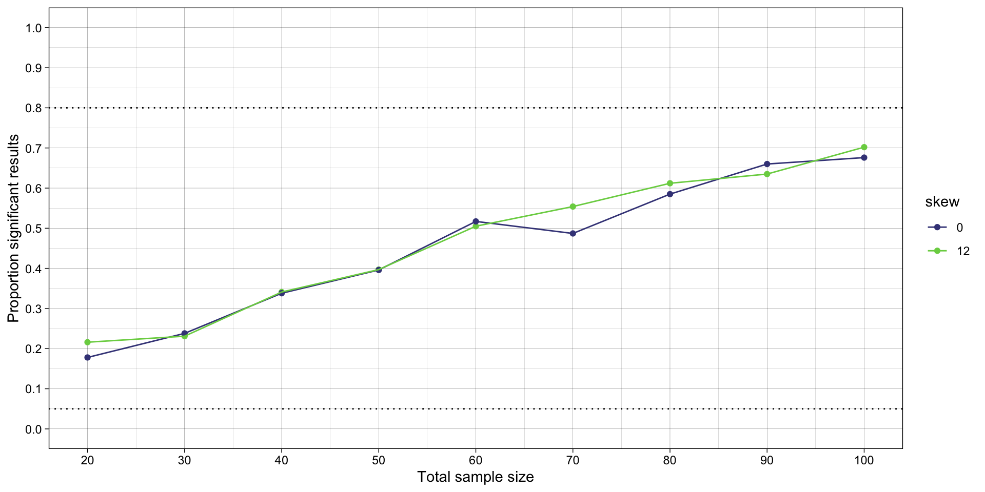
## Power of Student's t-test
Code taken from the previous lesson, with some simplifications.
```{r fig.height=5, fig.width=10}
# define data generating function ----
generate_data <- function(n,
                          location_control, # location, akin to mean
                          location_intervention,
                          scale, # scale, akin to SD
                          skew) { # slant/skew. When 0, produces normal/gaussian data

  data_control <-
    tibble(condition = "control",
           score = rsn(n = n,
                       xi = location_control, # location, akin to mean
                       omega = scale, # scale, akin to SD
                       alpha = skew)) # slant/skew. When 0, produces normal/gaussian data

  data_intervention <-
    tibble(condition = "intervention",
           score = rsn(n = n,
                       xi = location_intervention, # location, akin to mean
                       omega = scale, # scale, akin to SD
                       alpha = skew)) # slant/skew. When 0, produces normal/gaussian data

  data <- bind_rows(data_control,
                    data_intervention)

  return(data)
}


# define data analysis function ----
analyze_data_students_t <- function(data) {

  hypothesis_test_students_t <- t.test(formula = score ~ condition,
                                       data = data,
                                       var.equal = TRUE,
                                       alternative = "two.sided")

  res <- tibble(hypothesis_test_p_students_t = hypothesis_test_students_t$p.value)

  return(res)
}

# define experiment parameters ----
experiment_parameters <- expand_grid(
  n = seq(from = 10, to = 50, by = 5),
  mean_control = 0,
  mean_intervention = 0.5,
  sd = 1,
  skew = c(0, 12),     # slant/skew. When 0, produces normal/gaussian data
  iteration = 1:1000
) |>
  # calculate skew-normal parameters
  # don't worry about the math, it's not important to understand
  mutate(delta = skew / sqrt(1 + skew^2),
         scale = sd / sqrt(1 - 2 * delta^2 / pi),
         location_control = mean_control - scale * delta * sqrt(2 / pi),
         location_intervention = mean_intervention - scale * delta * sqrt(2 / pi))


# run simulation ----
# results are cached to disk: the simulation is only run the first time, and read back
# in on subsequent renders. delete the .rds file if you change the simulation code.
dir.create("results", showWarnings = FALSE)

if(file.exists("results/simulation_conditional_tests_1.rds")){

  simulation <- read_rds("results/simulation_conditional_tests_1.rds")

} else {

  set.seed(42)

  simulation <-
    # using the experiment parameters
    experiment_parameters |>

    # shuffle the rows of the grid to load balance the computationally expensive
    # iterations evenly across the workers
    slice_sample(prop = 1) |>

    # generate data using the data generating function and the parameters relevant to data generation
    mutate(generated_data = future_pmap(.l = list(n = n,
                                                  location_control = location_control,
                                                  location_intervention = location_intervention,
                                                  scale = scale,
                                                  skew = skew),
                                        .f = generate_data,
                                        .progress = TRUE,
                                        .options = furrr_options(seed = TRUE))) |>

    # apply the analysis function to the generated data using the parameters relevant to analysis
    mutate(analysis_results_students_t = future_pmap(.l = list(data = generated_data),
                                                     .f = analyze_data_students_t,
                                                     .progress = TRUE,
                                                     .options = furrr_options(seed = TRUE))) |>

    # undo the shuffle so the rows are back in the order of the experiment grid
    arrange(n, skew, iteration) |>

    # the generated data sets are not needed after they have been analyzed, and keeping
    # them would make the saved file enormous
    select(-generated_data)

  write_rds(x = simulation,
            file = "results/simulation_conditional_tests_1.rds",
            compress = "gz")

}

# summarise simulation results over the iterations ----
## ie what proportion of p values are significant (< .05)
simulation_summary <- simulation |>
  unnest(analysis_results_students_t) |>
  mutate(skew = as.factor(skew)) |>
  group_by(n,
           location_control,
           location_intervention,
           scale,
           skew) |>
  # rather than calculating the proportion of significant results by hand, use
  # {simhelpers}'s dedicated function for the empirical rejection rate.
  # calc_rejection() also returns the number of iterations and the Monte Carlo Standard
  # Error of the rate; select() keeps and renames just the rate itself
  reframe(calc_rejection(data     = pick(everything()),
                         p_values = hypothesis_test_p_students_t,
                         alpha    = 0.05) |>
            select(proportion_significant_students_t = rej_rate))

# plot
ggplot(simulation_summary, aes(n*2, proportion_significant_students_t, color = skew)) +
  geom_hline(yintercept = 0.80, linetype = "dotted") +
  geom_hline(yintercept = 0.05, linetype = "dotted") +
  geom_point() +
  geom_line() +
  scale_x_continuous(breaks = breaks_pretty(n = 9), name = "Total sample size") +
  scale_y_continuous(limits = c(0, 1), breaks = breaks_pretty(n = 9), name = "Proportion significant results") +
  theme_linedraw() +
  scale_color_viridis_d(begin = 0.2, end = 0.8)
```
## Power of Student's t-test vs. Wilcoxon rank-sum test
Aka Mann-Whitney U-test.
### Exercise
Write a function called `analyze_data_wilcox()` that uses `wilcox.test()` instead of `t.test()` to compare the differences in central tendency between the conditions.
Have it return a data frame with a p value called `hypothesis_test_p_wilcox`.
```{r}
```
### Simulation
```{r}
#| eval: false # once you've written the functions, you can remove this to run the code
# results are cached to disk: the simulation is only run the first time, and read back
# in on subsequent renders. delete the .rds file if you change the simulation code.
dir.create("results", showWarnings = FALSE)

if(file.exists("results/simulation_conditional_tests_2.rds")){

  simulation <- read_rds("results/simulation_conditional_tests_2.rds")

} else {

  set.seed(42)

  simulation <-
    # using the experiment parameters
    experiment_parameters |>

    # shuffle the rows of the grid to load balance the computationally expensive
    # iterations evenly across the workers
    slice_sample(prop = 1) |>

    # generate data using the data generating function and the parameters relevant to data generation
    mutate(generated_data = future_pmap(.l = list(n = n,
                                                  location_control = location_control,
                                                  location_intervention = location_intervention,
                                                  scale = scale,
                                                  skew = skew),
                                        .f = generate_data,
                                        .progress = TRUE,
                                        .options = furrr_options(seed = TRUE))) |>

    # analyze data with students t test
    mutate(analysis_results_students_t = future_pmap(.l = list(data = generated_data),
                                                     .f = analyze_data_students_t,
                                                     .progress = TRUE,
                                                     .options = furrr_options(seed = TRUE))) |>

    # analyze data with wilcox t test
    mutate(analysis_results_wilcox = future_pmap(.l = list(data = generated_data),
                                                 .f = analyze_data_wilcox,
                                                 .progress = TRUE,
                                                 .options = furrr_options(seed = TRUE))) |>

    # undo the shuffle so the rows are back in the order of the experiment grid
    arrange(n, skew, iteration) |>

    # the generated data sets are not needed after they have been analyzed, and keeping
    # them would make the saved file enormous
    select(-generated_data)

  write_rds(x = simulation,
            file = "results/simulation_conditional_tests_2.rds",
            compress = "gz")

}
```
```{r fig.height=5, fig.width=10}
#| eval: false # once you've written the functions, you can remove this to run the code
# summarise simulation results over the iterations ----
## ie what proportion of p values are significant (< .05)
simulation_summary <- simulation |>
  unnest(analysis_results_students_t) |>
  unnest(analysis_results_wilcox) |>
  mutate(skew = as.factor(skew)) |>
  group_by(n,
           location_control,
           location_intervention,
           scale,
           skew) |>
  # {simhelpers}'s dedicated function for the empirical rejection rate, applied to each
  # test's p values. select() keeps and renames just the rate itself
  reframe(calc_rejection(data     = pick(everything()),
                         p_values = hypothesis_test_p_students_t,
                         alpha    = 0.05) |>
            select(proportion_significant_students_t = rej_rate),
          calc_rejection(data     = pick(everything()),
                         p_values = hypothesis_test_p_wilcox,
                         alpha    = 0.05) |>
            select(proportion_significant_wilcox = rej_rate))

# plots
ggplot(simulation_summary, aes(n*2, proportion_significant_students_t, color = skew)) +
  geom_hline(yintercept = 0.80, linetype = "dotted") +
  geom_hline(yintercept = 0.05, linetype = "dotted") +
  geom_point() +
  geom_line() +
  scale_x_continuous(breaks = breaks_pretty(n = 9), name = "Total sample size") +
  scale_y_continuous(limits = c(0, 1), breaks = breaks_pretty(n = 9), name = "Proportion significant results") +
  theme_linedraw() +
  scale_color_viridis_d(begin = 0.2, end = 0.8) +
  ggtitle("Power of Student's t-test for Cohen's d = 0.5")

ggplot(simulation_summary, aes(n*2, proportion_significant_wilcox, color = skew)) +
  geom_hline(yintercept = 0.80, linetype = "dotted") +
  geom_hline(yintercept = 0.05, linetype = "dotted") +
  geom_point() +
  geom_line() +
  scale_x_continuous(breaks = breaks_pretty(n = 9), name = "Total sample size") +
  scale_y_continuous(limits = c(0, 1), breaks = breaks_pretty(n = 9), name = "Proportion significant results") +
  theme_linedraw() +
  scale_color_viridis_d(begin = 0.2, end = 0.8) +
  ggtitle("Power of Wilcoxon rank-sum test for Cohen's d = 0.5")
```
- What's the upside and downside of each?
## Power of Shapiro-Wilk's test with skew-normal data
### Exercise
Write a function called `test_assumption_of_normality()` that uses `shapiro.test()` to assess for non-normality in each condition (control and intervention). It should return a p value for both tests.
You can use `filter()` and `pull()` to extract the scores for each condition and test them separately for normality. Return the lower of the two p values as `assumption_test_p_sharpirowilks_lower`.
```{r}
```
### Simulation
Test for normality in each of two samples, and return a decision of non-normality if it is found in either.
```{r fig.height=5, fig.width=10}
#| eval: false # once you've written the functions, you can remove this to run the code
# results are cached to disk: the simulation is only run the first time, and read back
# in on subsequent renders. delete the .rds file if you change the simulation code.
dir.create("results", showWarnings = FALSE)

if(file.exists("results/simulation_conditional_tests_3.rds")){

  simulation <- read_rds("results/simulation_conditional_tests_3.rds")

} else {

  set.seed(42)

  simulation <-
    # using the experiment parameters
    experiment_parameters |>

    # shuffle the rows of the grid to load balance the computationally expensive
    # iterations evenly across the workers
    slice_sample(prop = 1) |>

    # generate data using the data generating function and the parameters relevant to data generation
    mutate(generated_data = future_pmap(.l = list(n = n,
                                                  location_control = location_control,
                                                  location_intervention = location_intervention,
                                                  scale = scale,
                                                  skew = skew),
                                        .f = generate_data,
                                        .progress = TRUE,
                                        .options = furrr_options(seed = TRUE))) |>

    # analyze data with students t test
    mutate(analysis_results_students_t = future_pmap(.l = list(data = generated_data),
                                                     .f = analyze_data_students_t,
                                                     .progress = TRUE,
                                                     .options = furrr_options(seed = TRUE))) |>

    # analyze data with wilcox t test
    mutate(analysis_results_wilcox = future_pmap(.l = list(data = generated_data),
                                                 .f = analyze_data_wilcox,
                                                 .progress = TRUE,
                                                 .options = furrr_options(seed = TRUE))) |>

    # apply the analysis function to the generated data using the parameters relevant to analysis
    mutate(analysis_results_normality = future_pmap(.l = list(data = generated_data),
                                                    .f = test_assumption_of_normality,
                                                    .progress = TRUE,
                                                    .options = furrr_options(seed = TRUE))) |>

    # undo the shuffle so the rows are back in the order of the experiment grid
    arrange(n, skew, iteration) |>

    # the generated data sets are not needed after they have been analyzed, and keeping
    # them would make the saved file enormous
    select(-generated_data)

  write_rds(x = simulation,
            file = "results/simulation_conditional_tests_3.rds",
            compress = "gz")

}

# summarise simulation results over the iterations ----
## ie what proportion of p values are significant (< .05)
simulation_summary <- simulation |>
  unnest(analysis_results_students_t) |>
  unnest(analysis_results_wilcox) |>
  unnest(analysis_results_normality) |>
  mutate(skew = as.factor(skew)) |>
  group_by(n,
           location_control,
           location_intervention,
           scale,
           skew) |>
  # {simhelpers}'s dedicated function for the empirical rejection rate, applied to the
  # p values of each hypothesis test and of the assumption test. select() keeps and
  # renames just the rate itself
  reframe(calc_rejection(data     = pick(everything()),
                         p_values = hypothesis_test_p_students_t,
                         alpha    = 0.05) |>
            select(proportion_significant_students_t = rej_rate),
          calc_rejection(data     = pick(everything()),
                         p_values = hypothesis_test_p_wilcox,
                         alpha    = 0.05) |>
            select(proportion_significant_wilcox = rej_rate),
          calc_rejection(data     = pick(everything()),
                         p_values = assumption_test_p_sharpirowilks_lower,
                         alpha    = 0.05) |>
            select(proportion_significant_shapirowilks = rej_rate))

# plot
ggplot(simulation_summary, aes(n*2, proportion_significant_shapirowilks, color = skew)) +
  geom_hline(yintercept = 0.80, linetype = "dotted") +
  geom_hline(yintercept = 0.05, linetype = "dotted") +
  geom_point() +
  geom_line() +
  scale_x_continuous(breaks = breaks_pretty(n = 9), name = "Total sample size") +
  scale_y_continuous(limits = c(0, 1), breaks = breaks_pretty(n = 9), name = "Proportion significant results") +
  theme_linedraw() +
  scale_color_viridis_d(begin = 0.2, end = 0.8) +
  ggtitle("Power of Shapiro-Wilks test applied to each condition")
```
- What does this tell us?
## Conditionally running a Student's t-test or a Wilcoxon rank-sum test depending on Shapiro-Wilk's test for normality in both samples
I.e., for each iteration, we calculate a conditional p value: if either of the Shapiro-Wilks tests are significant (evidence of non-normality), use the p value from the Wilcox test; if not, use the Student's t test's p value.
We then summarize the power of the conditional p value vs. the Wilcox's test's p value. This compares the workflows where we either:
a) use Shapiro-Wilk's tests to choose which method to use to test the hypothesis
b) just use the non-parametric test by default.
```{r}
#| code-fold: true
#| fig.height: 5
#| fig.width: 10
#| eval: false # once you've written the functions, you can remove this to run the code
# summarise simulation results over the iterations ----
simulation_summary <- simulation |>
  unnest(analysis_results_students_t) |>
  unnest(analysis_results_wilcox) |>
  unnest(analysis_results_normality) |>
  # condition logic
  mutate(hypothesis_p_conditional = if_else(condition = assumption_test_p_sharpirowilks_lower < .05,
                                            true = hypothesis_test_p_wilcox,
                                            false = hypothesis_test_p_students_t)) |>
  # summarize
  mutate(skew = as.factor(skew)) |>
  group_by(n,
           mean_control,
           mean_intervention,
           scale,
           skew) |>
  # {simhelpers}'s dedicated function for the empirical rejection rate, applied to each
  # workflow's p values. select() keeps and renames just the rate itself
  reframe(calc_rejection(data     = pick(everything()),
                         p_values = hypothesis_p_conditional,
                         alpha    = 0.05) |>
            select(proportion_significant_conditional = rej_rate),
          calc_rejection(data     = pick(everything()),
                         p_values = hypothesis_test_p_students_t,
                         alpha    = 0.05) |>
            select(proportion_significant_students_t = rej_rate),
          calc_rejection(data     = pick(everything()),
                         p_values = hypothesis_test_p_wilcox,
                         alpha    = 0.05) |>
            select(proportion_significant_wilcox = rej_rate)) |>
  mutate(power_diff = proportion_significant_conditional - proportion_significant_wilcox)

# plots
simulation_summary |>
  pivot_longer(cols = c(proportion_significant_conditional,
                        proportion_significant_students_t,
                        proportion_significant_wilcox),
               names_to = "test",
               values_to = "empirical_detection_rate") |>
  mutate(test = str_remove(test, "proportion_significant_")) |>
  ggplot(aes(x = n*2,
             y = empirical_detection_rate,
             group = test,
             color = test)) +
  geom_hline(yintercept = 0.80, linetype = "dotted") +
  geom_hline(yintercept = 0.05, linetype = "dotted") +
  geom_line() +
  geom_point() +
  scale_x_continuous(breaks = breaks_pretty(n = 9), name = "Total sample size") +
  scale_y_continuous(limits = c(0, 1), breaks = breaks_pretty(n = 9), name = "Proportion significant results") +
  theme_linedraw() +
  scale_color_viridis_d(begin = 0.2, end = 0.8) +
  ggtitle("Power of conditional-Student's or Wilcox test vs. default-Wilcox test for Cohen's d = 0.5") +
  facet_wrap(~skew)
```
- What does this tell us about whether we should (a) test the assumption of normality and then run a (non)parameteric test conditionally or just run the non-parametric test by default?
- What interpretation issues might be an argument against doing this by default?
- Are you starting to see why statisticians usually reply with "it depends" when we ask them questions?
## Recap
What did you learn here?
- About statistical tests?
- About using Monte Carlo simulations to understand not just single tests but to understand workflows?
- About how to use this {purrr} simulation workflow to analyze data more than one way and make conditional decisions, in order to model the behavior of scientists?
## At-home exercises
### Collate the simulation above into a single code chunk with all the pieces to run the full simulation
I.e., all three data analysis mutate()s in one pipe, starting with the parameters.
```{r}
# paste necessary code in here
```
### Elaborate the simulation
Right now the simulation only examines a fixed population effect size (0 or .5). Perhaps the supposed negative impact of violating normality would be seen at other effect sizes? Perhaps other values of skew would generate different results - how skewed is skew=12? Vary this or indeed other things to make an informed decision about how to choose which test(s) to run to make the inference about differences in means between conditions.
```{r}
```
### Develop a simulation to examine the power of the conditional use of (non)parametric based on heteroscedasticity vs using non-parametric tests by default
Decisions about which hypothesis test is used are also made on the basis of other tests of those assumptions. For example, heteroscedasticity (equal SDs) can be tested using `leveneTest()`. This has lower power than Bartlett's test but does not assume normality.
Write a simulation that is analogous to the one above, but which compares the statistical power of a) the conditional use of Student's t test or Wilcox test based on the result of Levene's test vs. b) using Wilcox test by default.
For simplicity:
- Use a true effect population effect size of Cohen's d = 0.5 in all simulations.
- Use only normal data.
- Vary degree of heteroscedasticity between the groups, i.e., set it to 1, 1.5, or 2 in the intervention group. Work out what you'll need to set it to in the control group and why.
- Use the same sample sizes as as in the above simulation (i.e., `n = c(10, 25, 50, 100, 200)`).
```{r}
#| eval: FALSE
#| include: FALSE
```