# Foundation concepts <span class="badge badge-draft3">✎ Polishing</span>
```{r}
#| include: false
# if it is available, run the setup script that tells quarto to round all df/tibble outputs to three decimal places
if(file.exists("../_setup.R")){source("../_setup.R")}
```
```{r}
#| include: false
library(roundwork)
library(ggplot2)
library(scales)
library(dplyr)
library(tidyr)
library(purrr)
set.seed(42)
```
## Why do we use simulation?
Imagine you're throwing yourself a birthday party, and need to buy food and drinks for everyone who is coming. First of all: happy birthday! Second of all: you probably need to figure out _how much_ food and drink to buy in order to make sure everybody has enough to eat and enough to drink. At the same time, you're not made of money, so you probably don't want to buy too much, either.
In this scenario, you probably will consider some hypothetical possibilities to help you estimate how much food and drink you'll need. You might think: well, if 20 people come, and they eat an average of half a pizza each, plus 4 bottles of soda each, then we'll probably need 20 * .5 = 10 pizzas, and 20 * 4 = 80 bottles. Easy!
But wait - your best friend is coming, and she always eats at least one and a half full pizzas by herself! Plus maybe some people will have already eaten before they arrive. Some people are also going to another party after yours finishes, so they might not stay that long, so maybe they won't drink as much as you expect. And maybe fewer than 20 people will show up! Or more! How could we plan for this when there is so much uncertainty?
Using simple averages like we did above is easy, but it's imperfect. So, using your statistics training, you decide to figure out the _distribution_ of food and drink consumption, as well the number of attendees. So you think: OK, I think people will eat pizzas and drink bottles following normal distributions. People will eat an average of 0.5 pizzas, with a standard deviation of 0.1 pizzas. And people will drink 4 bottles, with a standard deviation of 1 bottle. Then you think the same about attendees: on average 20 people will come, with a standard deviation of 2 people. Great!
Except...what do you do with this information? These distributions are interesting, and maybe even correct, but how can we translate this into an actionable decision about how much food and drink you should buy for your party?
Well, what if you threw 100 parties with the means and SDs for food, drink, and attendance above? In such a case, you could figure out some smart way of how much to buy. For example, you could say: I will buy enough food and drink to ensure that, in 95 out of those 100 parties, I would have enough for everyone.
This is one of the many, many scenarios that we can use simulation for. When we can make decent guesses about statistical properties of possible scenarios (like how much food and drink people will consume, and how many people will show up at the party) then we can generate possible scenarios many times using these statistical properties, and then make inferences about the things we care about (in this case, how much food and drink to buy). Simulation can extend far beyond simple applications like this - we use it to ensure that production lines in factories run smoothly; to ensure that products are functioning effectively, and XXX.
You will learn all about how, when, and why to use simulation in this course. For now, let's get an answer to our party question. You won't know what's happening in the code right now - that's OK. We will build up your understanding over the following chapters so that you can come back and easily understand this. For now:
```{r}
# set seed
set.seed(2026)

# Design experiment
experiment_parameters <- expand_grid(
  party_number = 1:100,
  mean_number_of_attendees = 20,
  sd_number_of_attendees = 2,
  mean_pizza_eaten = 0.5,
  sd_pizza_eaten = 0.1,
  mean_bottles_drank = 4,
  sd_bottles_drank = 1
)

# Generate data function
generate_data <- function(mean_number_of_attendees,
                          sd_number_of_attendees,
                          mean_pizza_eaten,
                          sd_pizza_eaten,
                          mean_bottles_drank,
                          sd_bottles_drank) {

  number_of_attendees <- rnorm(1, mean_number_of_attendees, sd_number_of_attendees)

  dat <- tibble(
    attendee = c(1:number_of_attendees),
    pizzas_eaten = round(rnorm(number_of_attendees, mean_pizza_eaten, sd_pizza_eaten), 1),
    bottles_drank = round(rnorm(number_of_attendees, mean_bottles_drank, sd_bottles_drank), 0)
  )

  dat

}


# analyze data function
analyze_data <- function(dat) {

  tibble(
    total_pizza_eaten = sum(dat$pizzas_eaten),
    total_bottles_drank = sum(dat$bottles_drank)
  )

}

# Run the experiment many times
simulation_results <- experiment_parameters |>
  mutate(
    generated_data = pmap(
      .l = list(
        mean_number_of_attendees,
        sd_number_of_attendees,
        mean_pizza_eaten,
        sd_pizza_eaten,
        mean_bottles_drank,
        sd_bottles_drank),
      .f = generate_data
      ),
    results = map(generated_data, analyze_data)
  ) |>
  unnest(results)


# summarise results
simulation_results |>
  summarise(
    pizzas_required = quantile(total_pizza_eaten, .95),
    bottles_required = quantile(total_bottles_drank, .95)
    )
```
To make sure that 95 out of 100 parties would be covered, we would need 12 pizzas and 93 bottles of beer!
## How are simulations different from studies?
In the party example above, we didn’t actually throw 100 birthday parties. We pretended to, using a few assumptions about what parties tend to look like (how many people show up, how much they eat and drink). That’s the key difference:
- In a study, you collect real data from the world.
- In a simulation, you generate fake-but-plausible data from a model of the world.
It might sound a bit strange to generate fake data to learn real things about the world. But this is exactly what makes simulation useful: it lets us explore "what would happen if...?" questions without having to pay for 100 parties, recruit 10,000 participants, or wait six months for data collection.
### A study learns from the world
In an empirical study, the world is the _data-generating process_. You don’t decide what the distribution of pizza consumption is — you discover it by measuring. Your sample contains surprises, messiness, measurement error, attrition, weird participants, and all the other things that make research both interesting and painful.
So the logic of a study is:
1. Collect data from the world.
2. Summarise and analyse that data.
3. Infer something about the process that produced it (and, hopefully, about the wider population).
Even when we use statistical models in studies, the model is our tool for learning from data we didn’t control.
### A simulation learns from your assumptions
In a simulation, you flip that around: the model is the data-generating process. You decide, in advance, what the distributions look like (or what mechanism produces the data). Then you generate many datasets from that mechanism, and try to understand what happens under those conditions.
So the logic of a simulation is:
1. Make experiments that assume things about how data are generated
2. Generate data under these assumptions
3. Analyse this dataset the same way you would analyse real data
4. Repeat this process many times
5. Summarise the results across datasets and experiment conditions
This is why simulation is sometimes described as doing statistics "in a sandbox": you control the world, and you watch what your analysis does inside it.
### Are simulations just making things up?
Yes! But not randomly. A simulation is only as good as the assumptions you put in. If you assume pizza consumption is normally distributed, you will generate a world where negative pizza consumption is theoretically possible. If you assume attendance varies with a standard deviation of 2, you’re asserting that wildly different attendance (say, 5 people or 60 people) is extremely unlikely.
And this is the point: simulation forces you to think about what processes might generate data.
A useful way to think about it is:
- A study asks: “What is true in the world?”
- A simulation asks: “If the world worked like this, what would happen?”
We use simulation because many questions we care about are hard to answer directly with studies. For example:
- If I run this analysis on data like mine, how often will I get a false positive?
- How much sample size do I need for reasonable power in my design (not in a textbook idealisation)?
- If I use method A vs method B, which one is more biased under realistic conditions?
- If participants drop out in a certain way, how badly does it distort my results?
- What is the distribution of a p-value under the null hypothesis?
You can’t usually run a real study thousands of times under controlled conditions to find out. But you can simulate it.
### Simulations don’t replace studies
Simulation is not a substitute for collecting data. It’s a tool for understanding methods, designing studies, stress-testing assumptions, and building intuition about uncertainty.
In the party example, simulation helped you make a decision given uncertainty — but the quality of that decision depended on whether your guessed means and standard deviations were sensible. If your friends are secretly world champion pizza-eaters and eat 3 pizzas each, your simulation will confidently recommend the wrong amount of pizza to buy
In short: studies are messy but grounded in reality; simulations are clean but grounded in assumptions.
## Key components of a Monte Carlo simulation study
Monte Carlo simulation studies are defined by the following key features:
1. Construct an experiment
2. Generate data
3. Analyze data
4. Repeat this many times
5. Summarize results over the experiment conditions
Future chapters will spell out in more detail what each one involves, but for the moment it is useful to rote learn them and repeat them to yourself. They serve two purposes. First, they are the best way to think about how a simulation actually works. Second, when we are writing code in this book, we will break it down in terms of each of these steps. Equally importantly for learners, errors or complications when learning to write simulations are, in my experience, very often due to inadequate separation of the steps. E.g., when your code does some data generation in the analysis block, or vice-versa.
To very briefly show you these components, we can build the code up in stages to create a very simple simulation answering "what is the distribution of *p*-values under the null hypothesis?"
### Construct an experiment
We plan to construct a simulation study experiment where data are sampled from two normally distributed populations with the no difference in means; to test for this difference in means using a Student's *t*-test's *p*-value; to do these generate-and-analyze steps many times; and to observe the distribution of *p*-values.
### Generate data
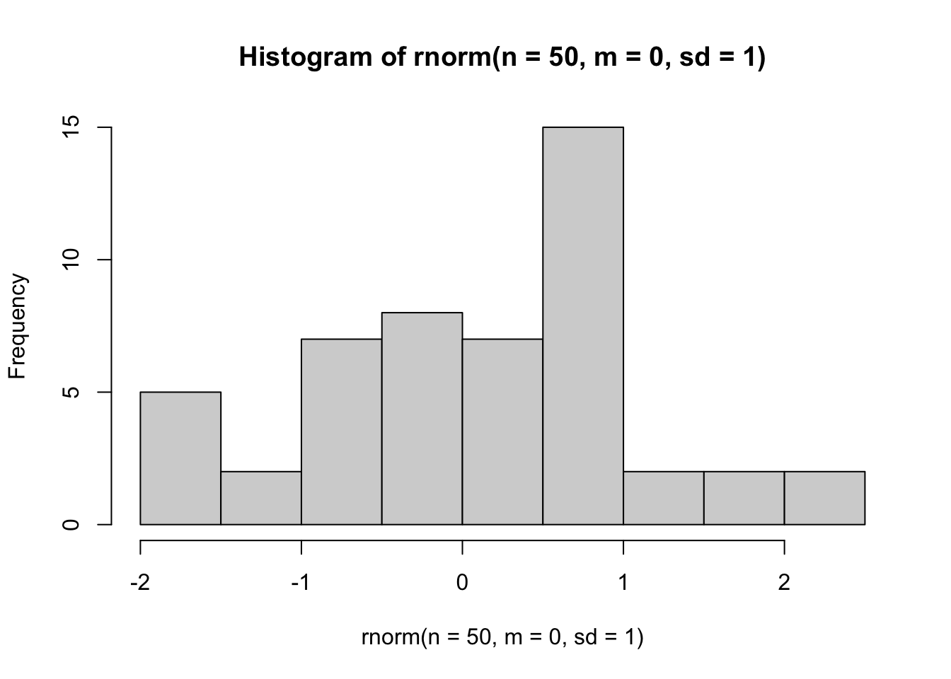
Draw data from a normally distributed population using `rnorm()` and plot it.
```{r}
rnorm(n = 50, m = 0, sd = 1) |>
  hist()
```
Now, we generate two normally distributed data sets and fit a Student's *t*-test.
Check your learning: In the code above, the population means in both samples are equivalent. What does a *t*-test test for? How does this choice of means implement a null population effect?
::: {.callout-note collapse="true" title="Click to show answer"}
*t*-tests allow us to make inferences about whether two population means differ.
While many of us are in the habit of simply saying the t-test "tests for differences", you'll learn in this course that it's much clearer and more precise to say that they (a) test for differences in means and (b) test for differences at the population level, not the sample. We can trivially say that the sample means are different or not depending on whether they're numerically identical or not. For example, if we observe the sample means $M_{intervention}$ = 3.11 and $M_{control}$ = 3.14, no statistical test is needed to see that the sample means are different. Whether or not the populations they are drawn from are likely to be different requires an inference test, such as a *t*-test.
The above code implements a null population effect, i.e., where the two populations have no differences in means between them, by using the same value for `m` in both `rnorm()` call (i.e., 0). Even though many of the samples that will be drawn from these populations will be numerically different, the populations they are drawn from do not differ in their means.
:::
### Analyse data
Generate two normally distributed data sets and fit a *t*-test and extract the *p*-value
```{r}
t.test(x = rnorm(n = 50, m = 0, sd = 1),
       y = rnorm(n = 50, m = 0, sd = 1),
       var.equal = TRUE)
```
```{r}
t.test(x = rnorm(n = 50, m = 0, sd = 1),
       y = rnorm(n = 50, m = 0, sd = 1),
       var.equal = TRUE)$p.value
```
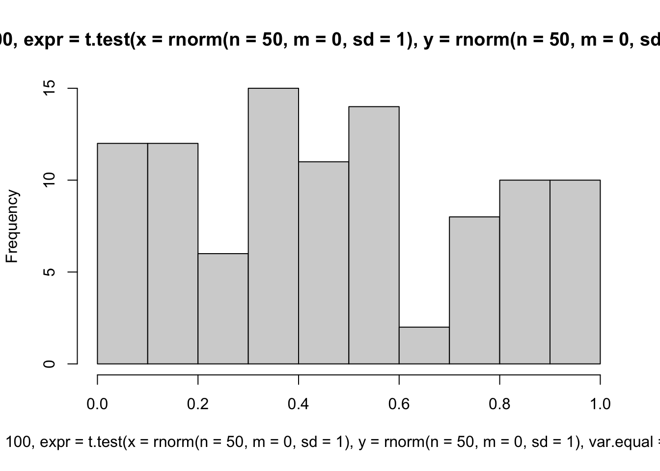
### Repeat this many times and summarize results
We repeat this using the `replicate()` function, and summarize across the iterations by plotting the *p*-values using `hist()`.
```{r}
replicate(n = 100,
          expr = t.test(x = rnorm(n = 50, m = 0, sd = 1),
                        y = rnorm(n = 50, m = 0, sd = 1),
                        var.equal = TRUE)$p.value) |>
  hist()
```
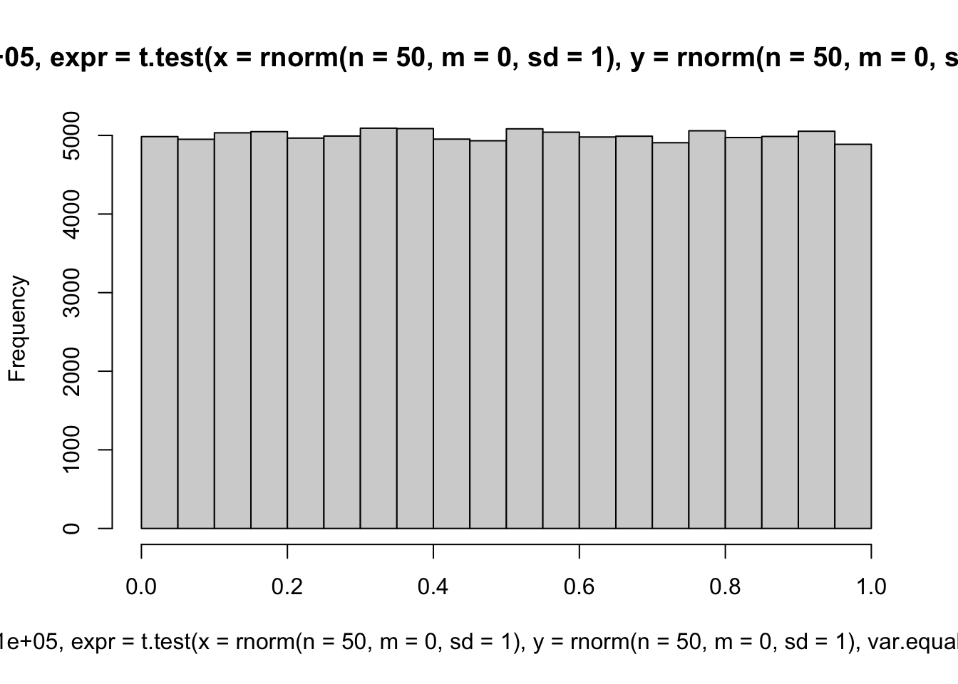
Next we increase the number of iterations, i.e., the number of times we repeat the generate-and-analyze steps.
```{r}
replicate(n = 100000,
          expr = t.test(x = rnorm(n = 50, m = 0, sd = 1),
                        y = rnorm(n = 50, m = 0, sd = 1),
                        var.equal = TRUE)$p.value) |>
  hist()
```
Check your learning: Why is the distribution more uniform when the number of iterations is higher?
::: {.callout-note collapse="true" title="Click to show answer"}
Just like in real-world studies, the number of samples from the population influences how stable the estimates are. The distribution of p-values in the smaple is only pefectly uniform when sample size is infinite. So, as simulated sample size increases, the uniformity of the distribution of p-values will generally increase.
:::
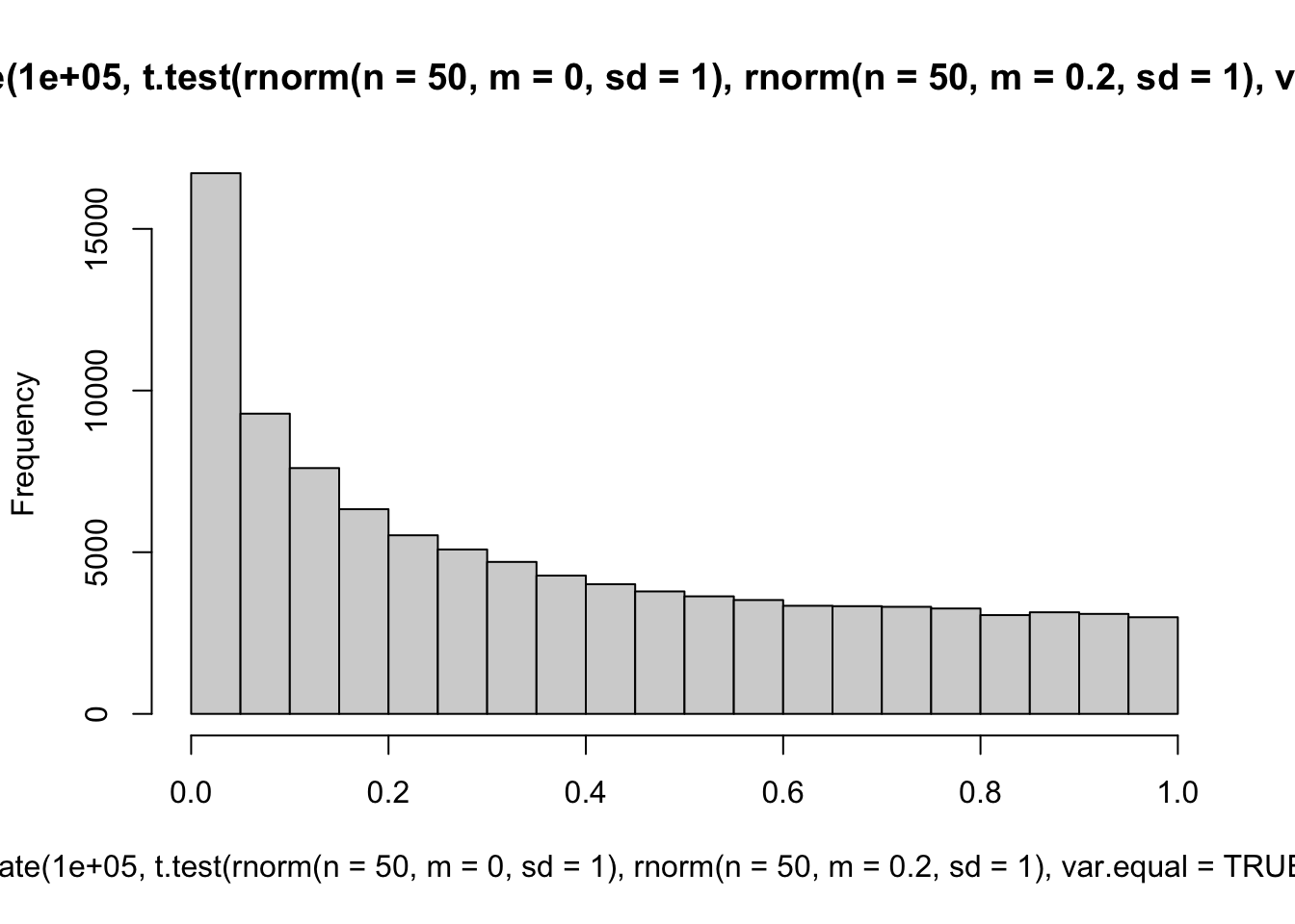
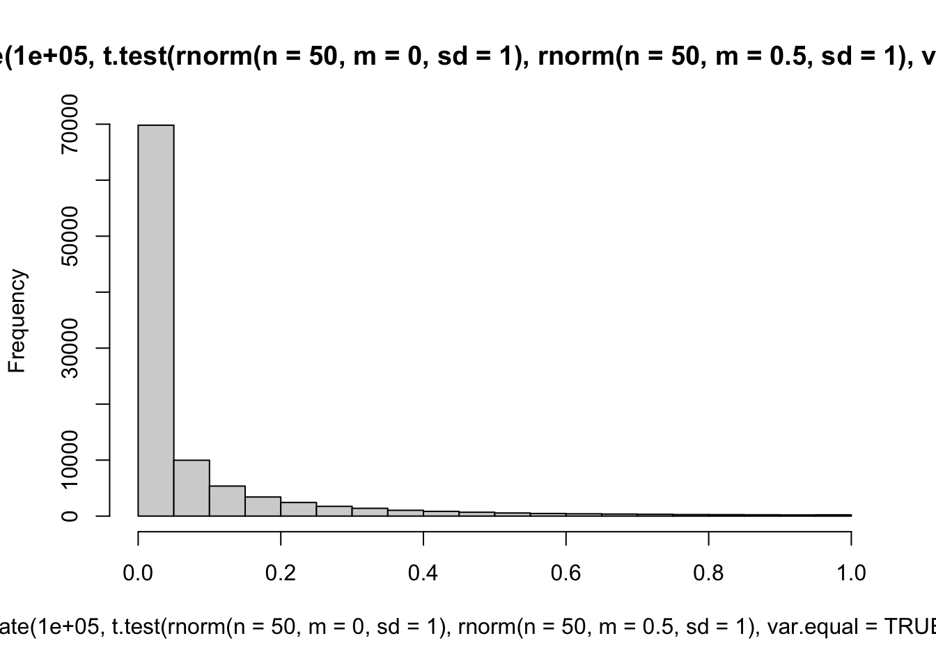
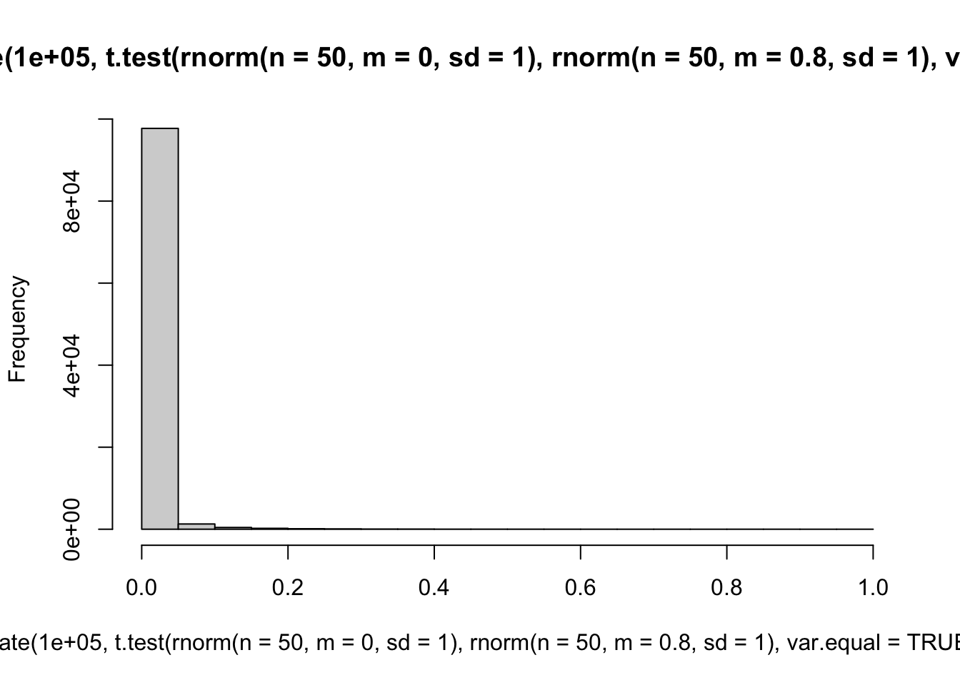
## Compare with distribution of *p*-values when population means are not equal
'Small', 'medium' and 'large' differences in population means.
```{r}
hist(replicate(100000, t.test(rnorm(n = 50, m = 0, sd = 1), rnorm(n = 50, m = 0.2, sd = 1), var.equal = TRUE)$p.value))
hist(replicate(100000, t.test(rnorm(n = 50, m = 0, sd = 1), rnorm(n = 50, m = 0.5, sd = 1), var.equal = TRUE)$p.value))
hist(replicate(100000, t.test(rnorm(n = 50, m = 0, sd = 1), rnorm(n = 50, m = 0.8, sd = 1), var.equal = TRUE)$p.value))
```
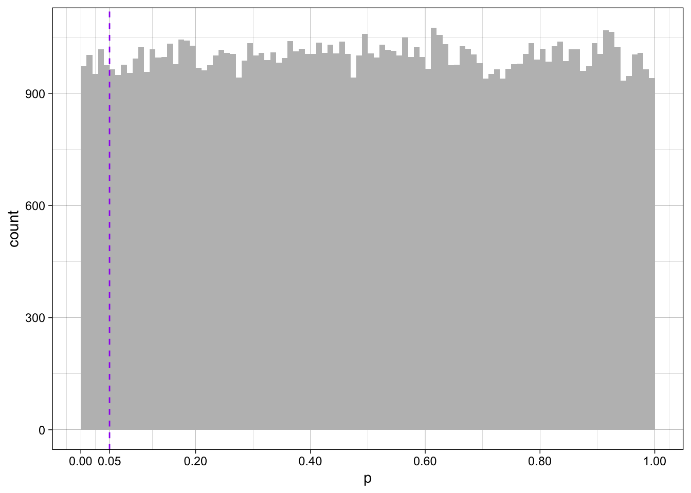
## What is the distribution of p values under the null hypothesis? [newer plotting]
```{r}
sim_h0 <- replicate(100000, t.test(rnorm(n = 500, m = 0, sd = 1), rnorm(n = 500, m = 0, sd = 1), var.equal = TRUE)$p.value)

percent_barely_sig_h0 <- round_up(mean(sim_h0 < .05 & sim_h0 > .02)*100, 1)

ggplot(data.frame(p = sim_h0), aes(p)) +
  geom_histogram(binwidth = 0.01, boundary = 0, fill = "grey") +
  scale_x_continuous(limits = c(0, 1), breaks = c(0, .05, .2, .4, .6, .8, 1)) +
  geom_vline(xintercept = 0.05, linetype = "dashed", color = "purple") +
  theme_linedraw()
```
In the long run of 100,000 studies with large sample sizes (N = 1000) and when the population effect size is zero (Cohen's d = 0), `r percent_barely_sig_h0`% of Student t-test *p*-values fall between .02 and .05.
This corresponds with the alpha value of the test, i.e., the *p* < .05 inference rule. When the population effect is zero, we will incorrectly conclude that it is non-zero in 5% of the long run of studies.
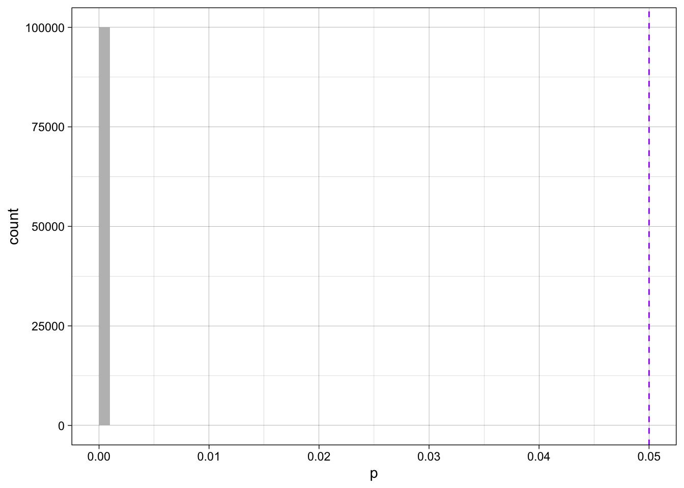
## How likely are barely significant *p*-values?
[A second simulation, to show their utility to raise as well as answer questions]
Many studies in the psychology literature report *p*-values between .02 and .05 ([Masicampo & Lalande, 2012](https://doi.org/10.1080/17470218.2012.7113); [Hartgerink et al., 2016](https://doi.org/10.7717/peerj.1935)). We can call these 'barely significant *p*-values'.
The common threshold for statistical significance, *p* < .05, treats all *p* values less than the threshold as equivalent. Regardless of whether your *p*-value is .048 or .000000000000000000001, the *p* <. 05 rule says you should conclude that there are detectable differences (e.g., differences in population means from a Student's *t*-test).
But is there a tipping point around .05 that makes this value particularly useful? Again, we could work through the math of it, but it is equally useful to simulate the long run of *p*-values and see how many are barely significant (.02 < p < .05). If they rarely occur, why do we use them in the rule?
```{r}
sim_h1 <- replicate(100000, t.test(rnorm(n = 500, m = 0, sd = 1), rnorm(n = 500, m = 0.8, sd = 1), var.equal = TRUE)$p.value)

percent_barely_sig_h1 <- round_up(mean(sim_h1 < .05 & sim_h1 > .02)*100, 1)

ggplot(data.frame(p = sim_h1), aes(p)) +
  geom_histogram(binwidth = 0.001, boundary = 0, fill = "grey") +
  scale_x_continuous(limits = c(0, 0.05), breaks = breaks_pretty(5)) +
  geom_vline(xintercept = 0.05, linetype = "dashed", color = "purple") +
  theme_linedraw()
```
In the long run of 100,000 studies with large sample sizes (N = 1000) and when the population effect size is large (Cohen's d = 0.8), `r percent_barely_sig_h1`% of Student t-test *p*-values fall between .02 and .05:
So, although the common statistical significance cut-off is 5% treats all *p*-values less than this equally, this quick simulation suggests that - to misquote George Orwell - some p-values are more equal than others.
But if barely significant *p*-values are rarely (or never) observed, why do we use *p* < .05 as the alpha value? Why not something lower, like .01, since it would decrease the number of false positives in the literature? This has certainly been argued for in the literature ([Benjamin et al., 2018](https://doi.org/10.1038/s41562-017-0189-z)). And, perhaps more worryingly, if they're so statistically rare, why do we see them so often in the literature?
The answers to these questions require us to dig deeper into *p*-values and what affects their distributions using more complicated simulations (e.g., [Maassen et al., 2025](https://doi.org/10.31234/osf.io/2uynm_v1); [Stefan & Schönbrodt, 2023](https://doi.org/10.1098/rsos.220346)). The take away message, for the moment, is that simulations can help give us pause for thought, help us check our own understanding, clarify our thinking, or answer meaningful questions - sometimes in only a few lines of code.
## Check your learning
#### What are the five core components of a Monte Carlo simulation?
::: {.callout-note collapse="true" title="Click to show answer"}
1. Construct an experiment
2. Generate data
3. Analyze data
4. Repeat these many times
5. Summarize results over the experiment conditions
:::
## TODO
- add content on positive and negative controls
- integrate some repetitive content below
- integrate information from slides, or the slides themselves
- remove old and new content redundancy