generate_data <- function(n_per_condition,
                          mean_control,
                          mean_intervention,
                          sd) {

  data_control <-
    tibble(condition = "control",
           score = rnorm(n = n_per_condition, mean = mean_control, sd = sd))

  data_intervention <-
    tibble(condition = "intervention",
           score = rnorm(n = n_per_condition, mean = mean_intervention, sd = sd))

  data_combined <- bind_rows(data_control,
                             data_intervention)

  return(data_combined)
}


# define data analysis function ----
analyze <- function(data) {

  students_ttest <- t.test(formula = score ~ condition,
                           data = data,
                           var.equal = TRUE,
                           alternative = "two.sided")

  res <- tibble(p = students_ttest$p.value)

  return(res)
}


# define experiment parameters ----
experiment_parameters <- expand_grid(
  n_per_condition = 100,
  mean_control = 0,
  mean_intervention = 0,
  sd = 1,
  iteration = 1:1000
)


# run simulation ----
# results are cached to disk: the simulation is only run the first time, and read back
# in on subsequent renders. delete the .rds file if you change the simulation code.
dir.create("results", showWarnings = FALSE)

if(file.exists("results/simulation_p_hacking_two_studies.rds")){

  simulation <- read_rds("results/simulation_p_hacking_two_studies.rds")

} else {

  set.seed(42)

  simulation <-
    # using the experiment parameters
    experiment_parameters |>

    # shuffle the rows of the grid to load balance the computationally expensive
    # iterations evenly across the workers
    slice_sample(prop = 1) |>

    # generate data using the data generating function and the parameters relevant to data generation
    mutate(generated_data_study1 = future_pmap(.l = list(n_per_condition = n_per_condition,
                                                         mean_control = mean_control,
                                                         mean_intervention = mean_intervention,
                                                         sd = sd),
                                               .f = generate_data,
                                               .progress = TRUE,
                                               .options = furrr_options(seed = TRUE))) |>
    mutate(generated_data_study2 = future_pmap(.l = list(n_per_condition = n_per_condition,
                                                         mean_control = mean_control,
                                                         mean_intervention = mean_intervention,
                                                         sd = sd),
                                               .f = generate_data,
                                               .progress = TRUE,
                                               .options = furrr_options(seed = TRUE))) |>

    # apply the analysis function to the generated data using the parameters relevant to analysis
    mutate(results_study1 = future_pmap(.l = list(data = generated_data_study1),
                                        .f = analyze,
                                        .progress = TRUE,
                                        .options = furrr_options(seed = TRUE))) |>
    mutate(results_study2 = future_pmap(.l = list(data = generated_data_study2),
                                        .f = analyze,
                                        .progress = TRUE,
                                        .options = furrr_options(seed = TRUE))) |>

    # undo the shuffle so the rows are back in the order of the experiment grid
    arrange(iteration) |>

    # the generated data sets are not needed after they have been analyzed, and keeping
    # them would make the saved file enormous
    select(-generated_data_study1, -generated_data_study2)

  write_rds(x = simulation,
            file = "results/simulation_p_hacking_two_studies.rds",
            compress = "gz")

}


# summarise simulation results over the iterations ----
simulation_summary <- simulation |>
  # unnest and rename
  unnest(results_study1) |>
  rename(p_study1 = p) |>
  unnest(results_study2) |>
  rename(p_study2 = p) |>
  # simulate flexible reporting
  mutate(p_hacked = ifelse(p_study1 < .05, p_study1, p_study2)) |>
  # summarize. rather than calculating the proportion of significant results by hand,
  # use {simhelpers}'s dedicated function for the empirical rejection rate.
  # calc_rejection() also returns the number of iterations and the Monte Carlo Standard
  # Error of the rate; select() keeps and renames just the rate itself
  reframe(calc_rejection(data     = pick(everything()),
                         p_values = p_study1,
                         alpha    = 0.05) |>
            select(prop_sig_study1 = rej_rate),
          calc_rejection(data     = pick(everything()),
                         p_values = p_study2,
                         alpha    = 0.05) |>
            select(prop_sig_study2 = rej_rate),
          calc_rejection(data     = pick(everything()),
                         p_values = p_hacked,
                         alpha    = 0.05) |>
            select(prop_sig_hacked = rej_rate)) |>
  pivot_longer(cols = everything(),
               names_to = "Source",
               values_to = "proportion_significant") |>
mutate(Source = str_remove(Source, "prop_sig_"))16 p-hacking via different forms of selecting reporting
16.1 Overview
p-hacking is increasing the false-positive rate through analytic choices. These choices are often a) flexible, in that many different options might be tried until significance is found (Gelman called this the “Garden of Forking Paths”), and b) undisclosed. However, it need not be either in a given instance: perhaps the very first analytic strategy tried produces the significant result (but if it hadn’t, other strategies would have been tried), or perhaps the author fully discloses the analytic choices but does not make clear to the reader how this undermines the severity of the test (i.e., it takes a very close reading to understand that the results present weak evidence, or the verbal conclusions oversell this).
p-hacking can occur because of the uniform distribution of p-values under the null hypothesis. Because all values are equally likely, you just have to keep rolling the dice to eventually find p < .05.
This lesson illustrates a few different examples of one broad form of p-hacking called selective reporting.
16.2 Selective reporting of studies
If I run two experiments, and only report the one that “works”, I will increase the false positive rate across studies. Perhaps it is because one really is better designed etc than the other. Or perhaps its just a false positive.
What would you guess the false positive rate is for two studies?
Let’s simulate it.
16.2.1 Run simulation
16.2.2 Results
simulation_summary |>
mutate_if(is.numeric, round_half_up, digits = 2) | Source | proportion_significant |
|---|---|
| study1 | 0.05 |
| study2 | 0.04 |
| hacked | 0.09 |
16.2.3 Conclusions
The false positive rate for two studies is ~10%, because each study has a 5% false positive rate.
See the exercises for this chapter to extend this simulation to four studies.
16.4 Selective reporting of correlated outcomes
Aka “outcome switching”, which is both common and problematic in clinical trials.
There are of course situations where the tests are not independent, and this makes it more complicated to understand the FPR. For example, imagine I am interested in the impact of CBT on depression, but I include multiple measures of depression and report the one that ‘worked’.
16.4.1 Generate correlated data
We haven’t simulated correlated data before so lets do that first.
set.seed(42)

dat <-
  faux::rnorm_multi(n = 1000,
                    mu = c(0, 0),
                    sd = c(1, 1),
                    r = -0.7,
                    varnames = c("var1", "var2"))

cor(dat)
var1 var2
var1 1.0000000 -0.7083632
var2 -0.7083632 1.0000000ggplot(dat, aes(var1, var2)) +
geom_point(alpha = 0.4) +
theme_linedraw()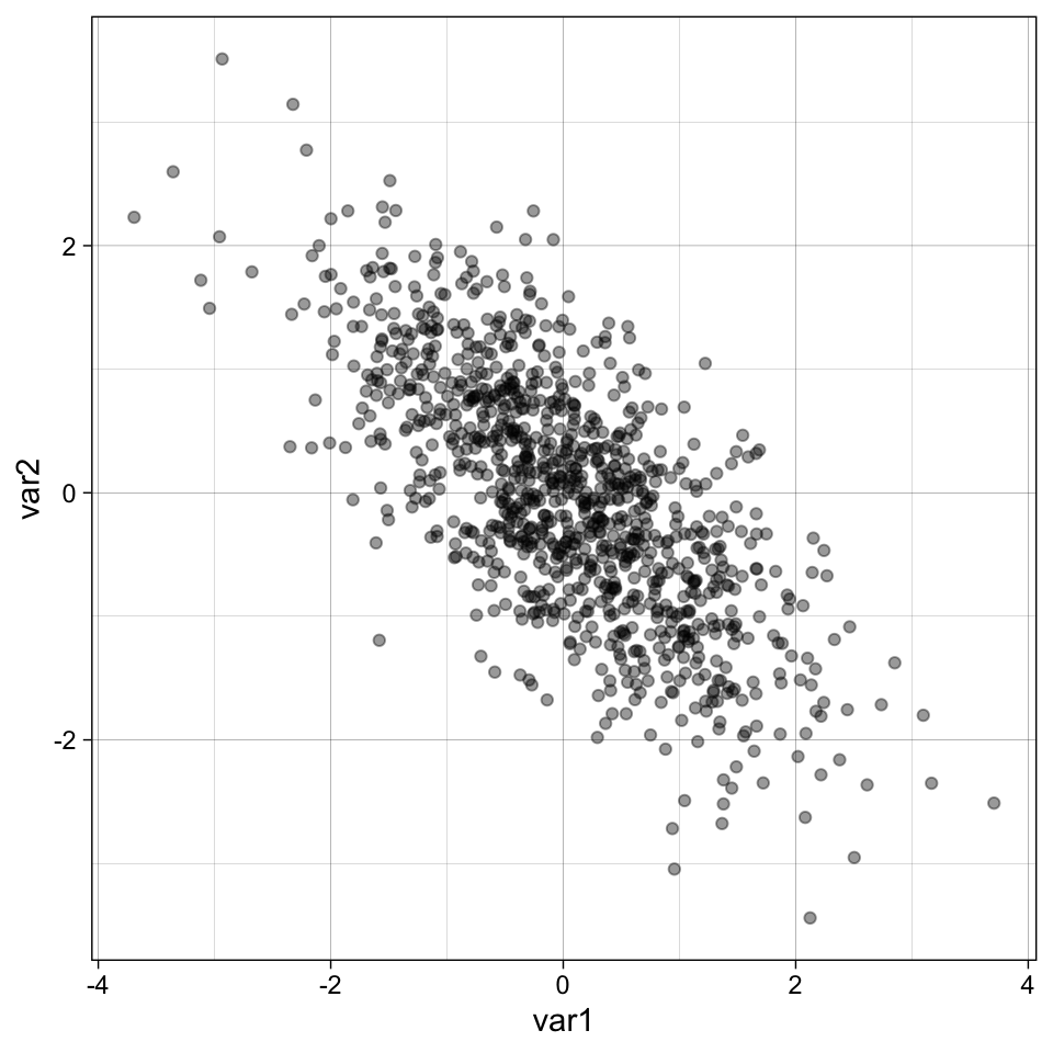
16.4.2 Generate data
Correlated outcomes, known groups differences.
generate_data <- function(n_per_condition,
                          r_between_outcomes,
                          mu_control, # vector of length 1 or k
                          mu_intervention, # vector of length 1 or k
                          sigma_control = 1, # vector of length 1 or k
                          sigma_intervention = 1) {  # vector of length 1 or k

  # generate data by condition
  data_control <-
    rnorm_multi(n = n_per_condition,
                mu = mu_control,
                sd = sigma_control,
                r = r_between_outcomes,
                varnames = c("outcome1", "outcome2", "outcome3")) |>
    mutate(condition = "Control")

  data_intervention <-
    rnorm_multi(n = n_per_condition,
                mu = mu_intervention,
                sd = sigma_intervention,
                r = r_between_outcomes,
                varnames = c("outcome1", "outcome2", "outcome3")) |>
    mutate(condition = "Intervention")

  # combine
  data_combined <-
    bind_rows(data_control,
              data_intervention) |>
    mutate(condition = fct_relevel(condition, "Intervention", "Control"))

  return(data_combined)
}
Check the function works
# simulate data
set.seed(42)

dat <- generate_data(n_per_condition = 100000,
                     r_between_outcomes = 0.6,
                     mu_control = 0,
                     mu_intervention = 1.5)

# parameter recovery
dat |>
  group_by(condition) |>
  summarize(mean_outcome1 = mean(outcome1),
            mean_outcome2 = mean(outcome2),
            correlation = cor(outcome1, outcome2)) |>
mutate_if(is.numeric, round_half_up, digits = 2)| condition | mean_outcome1 | mean_outcome2 | correlation |
|---|---|---|---|
| Intervention | 1.5 | 1.5 | 0.6 |
| Control | 0.0 | 0.0 | 0.6 |
16.4.3 Run simulation
# define data analysis function ----
analyze <- function(data, outcome) {

  # if you want to specify a column as an input, use rename()+{{}} to rename it before analysis
  data_renamed <- data |>
    rename(score = {{ outcome }})

  students_ttest <- t.test(formula = score ~ condition,
                           data = data_renamed,
                           var.equal = TRUE,
                           alternative = "two.sided")

  res <- tibble(p = students_ttest$p.value)

  return(res)
}


# define experiment parameters ----
experiment_parameters <- expand_grid(
  n_per_condition = 50,
  r_between_outcomes = c(0, .1, .2, .3, .4, .5, .6, .7, .8, .9, .99),
  mu_control = 0,
  mu_intervention = 0,
  iteration = 1:20000
)


# run simulation ----
# results are cached to disk: the simulation is only run the first time, and read back
# in on subsequent renders. delete the .rds file if you change the simulation code.
dir.create("results", showWarnings = FALSE)

if(file.exists("results/simulation_p_hacking_correlated_outcomes.rds")){

  simulation <- read_rds("results/simulation_p_hacking_correlated_outcomes.rds")

} else {

  set.seed(42)

  simulation <-
    # using the experiment parameters
    experiment_parameters |>

    # shuffle the rows of the grid to load balance the computationally expensive
    # iterations evenly across the workers
    slice_sample(prop = 1) |>

    # generate data using the data generating function and the parameters relevant to data generation
    mutate(generated_data = future_pmap(.l = list(n_per_condition = n_per_condition,
                                                  r_between_outcomes = r_between_outcomes,
                                                  mu_control = mu_control,
                                                  mu_intervention = mu_intervention),
                                        .f = generate_data,
                                        .progress = TRUE,
                                        .options = furrr_options(seed = TRUE))) |>

    # apply the analysis function to the generated data using the parameters relevant to analysis
    mutate(results_outcome1 = future_pmap(.l = list(data = generated_data,
                                                    outcome = "outcome1"),
                                          .f = analyze,
                                          .progress = TRUE,
                                          .options = furrr_options(seed = TRUE)),
           results_outcome2 = future_pmap(.l = list(data = generated_data,
                                                    outcome = "outcome2"),
                                          .f = analyze,
                                          .progress = TRUE,
                                          .options = furrr_options(seed = TRUE)),
           results_outcome3 = future_pmap(.l = list(data = generated_data,
                                                    outcome = "outcome3"),
                                          .f = analyze,
                                          .progress = TRUE,
                                          .options = furrr_options(seed = TRUE))) |>

    # unnest and rename
    unnest(results_outcome1) |>
    rename(outcome1_p = p) |>
    unnest(results_outcome2) |>
    rename(outcome2_p = p) |>
    unnest(results_outcome3) |>
    rename(outcome3_p = p) |>

    # undo the shuffle so the rows are back in the order of the experiment grid
    arrange(r_between_outcomes, iteration) |>

    # the generated data sets are not needed after they have been analyzed, and keeping
    # them would make the saved file enormous
    select(-generated_data)

  write_rds(x = simulation,
            file = "results/simulation_p_hacking_correlated_outcomes.rds",
            compress = "gz")

}


# summarise simulation results over the iterations ----
simulation_summary <- simulation |>
  # the smallest of the three p values: it is below alpha exactly when at least one of
  # the three outcomes was significant, i.e. it is the p value a researcher who switches
  # outcomes would report
  mutate(p_smallest = pmin(outcome1_p, outcome2_p, outcome3_p)) |>
  # summarize across iterations: empirical detection rates, using {simhelpers}'s
  # dedicated function for the empirical rejection rate
  group_by(n_per_condition,
           r_between_outcomes,
           mu_control,
           mu_intervention) |>
  reframe(calc_rejection(data = pick(everything()), p_values = outcome1_p, alpha = 0.05) |>
            select(prop_sig_outcome1 = rej_rate),
          calc_rejection(data = pick(everything()), p_values = outcome2_p, alpha = 0.05) |>
            select(prop_sig_outcome2 = rej_rate),
          calc_rejection(data = pick(everything()), p_values = outcome3_p, alpha = 0.05) |>
            select(prop_sig_outcome3 = rej_rate),
          calc_rejection(data = pick(everything()), p_values = p_smallest, alpha = 0.05) |>
            select(prop_sig_at_least_one = rej_rate))
16.4.4 Results
Empirical false positive rates as a function of the true correlation between outcomes. prop_sig_at_least_one is the empirical detection rate — the proportion of iterations in which at least one of the three outcomes reached p < .05, i.e. what a researcher who switches outcomes would report as “significant”.
simulation_summary |>
mutate_if(is.numeric, round_half_up, digits = 3)| n_per_condition | r_between_outcomes | mu_control | mu_intervention | prop_sig_outcome1 | prop_sig_outcome2 | prop_sig_outcome3 | prop_sig_at_least_one |
|---|---|---|---|---|---|---|---|
| 50 | 0.00 | 0 | 0 | 0.05 | 0.05 | 0.05 | 0.14 |
| 50 | 0.10 | 0 | 0 | 0.05 | 0.05 | 0.05 | 0.15 |
| 50 | 0.20 | 0 | 0 | 0.05 | 0.05 | 0.05 | 0.14 |
| 50 | 0.30 | 0 | 0 | 0.05 | 0.05 | 0.05 | 0.13 |
| 50 | 0.40 | 0 | 0 | 0.05 | 0.05 | 0.05 | 0.13 |
| 50 | 0.50 | 0 | 0 | 0.05 | 0.05 | 0.05 | 0.13 |
| 50 | 0.60 | 0 | 0 | 0.05 | 0.05 | 0.05 | 0.12 |
| 50 | 0.70 | 0 | 0 | 0.05 | 0.05 | 0.05 | 0.11 |
| 50 | 0.80 | 0 | 0 | 0.05 | 0.05 | 0.05 | 0.10 |
| 50 | 0.90 | 0 | 0 | 0.05 | 0.05 | 0.05 | 0.08 |
| 50 | 0.99 | 0 | 0 | 0.05 | 0.05 | 0.05 | 0.06 |
ggplot(simulation_summary, aes(r_between_outcomes, prop_sig_outcome1)) +
  geom_hline(yintercept = 0.05, linetype = "dotted") +
  geom_point() +
  geom_line() +
  scale_x_continuous(breaks = breaks_pretty(n = 9), name = "True correlation between outcomes") +
  scale_y_continuous(limits = c(0, .2), breaks = breaks_pretty(n = 5), name = "Empirical Detection Rate\n(outcome 1)") +
  theme_linedraw() +
  scale_color_viridis_d(begin = 0.2, end = 0.8)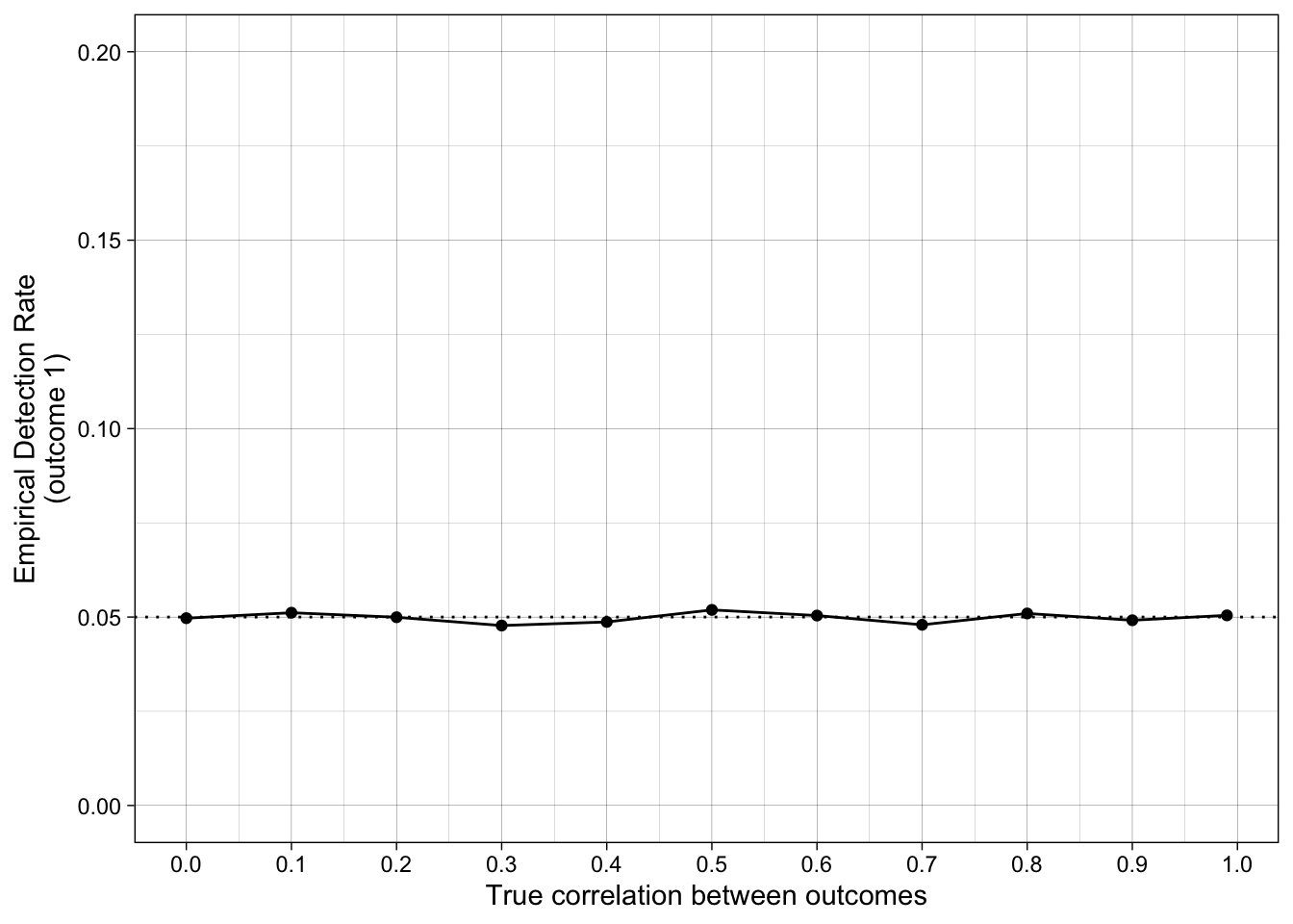
ggplot(simulation_summary, aes(r_between_outcomes, prop_sig_outcome2)) +
  geom_hline(yintercept = 0.05, linetype = "dotted") +
  geom_point() +
  geom_line() +
  scale_x_continuous(breaks = breaks_pretty(n = 9), name = "True correlation between outcomes") +
  scale_y_continuous(limits = c(0, .2), breaks = breaks_pretty(n = 5), name = "Empirical Detection Rate\n(outcome 2)") +
  theme_linedraw() +
  scale_color_viridis_d(begin = 0.2, end = 0.8)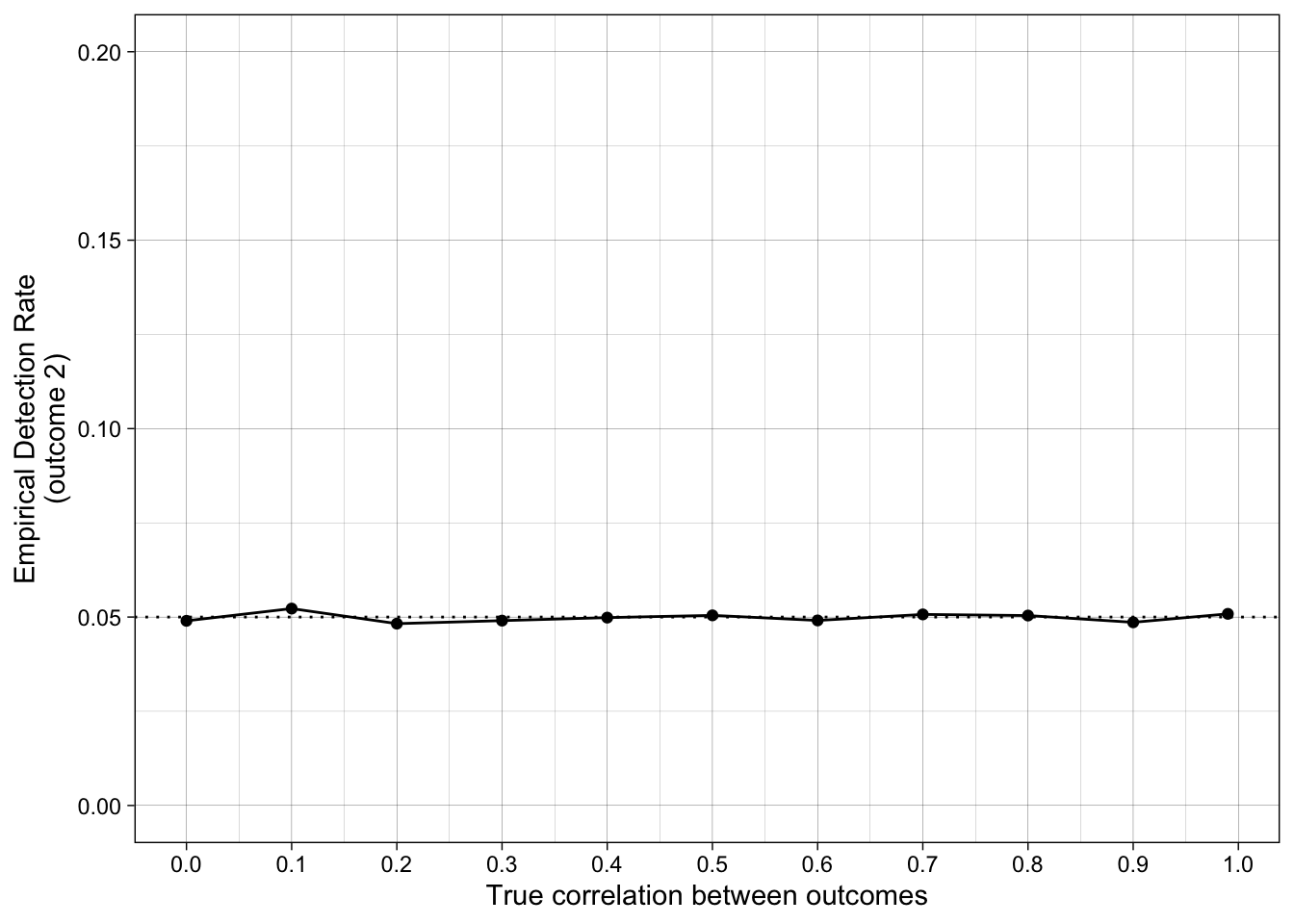
ggplot(simulation_summary, aes(r_between_outcomes, prop_sig_outcome3)) +
  geom_hline(yintercept = 0.05, linetype = "dotted") +
  geom_point() +
  geom_line() +
  scale_x_continuous(breaks = breaks_pretty(n = 9), name = "True correlation between outcomes") +
  scale_y_continuous(limits = c(0, .2), breaks = breaks_pretty(n = 5), name = "Empirical Detection Rate\n(outcome 3)") +
  theme_linedraw() +
  scale_color_viridis_d(begin = 0.2, end = 0.8)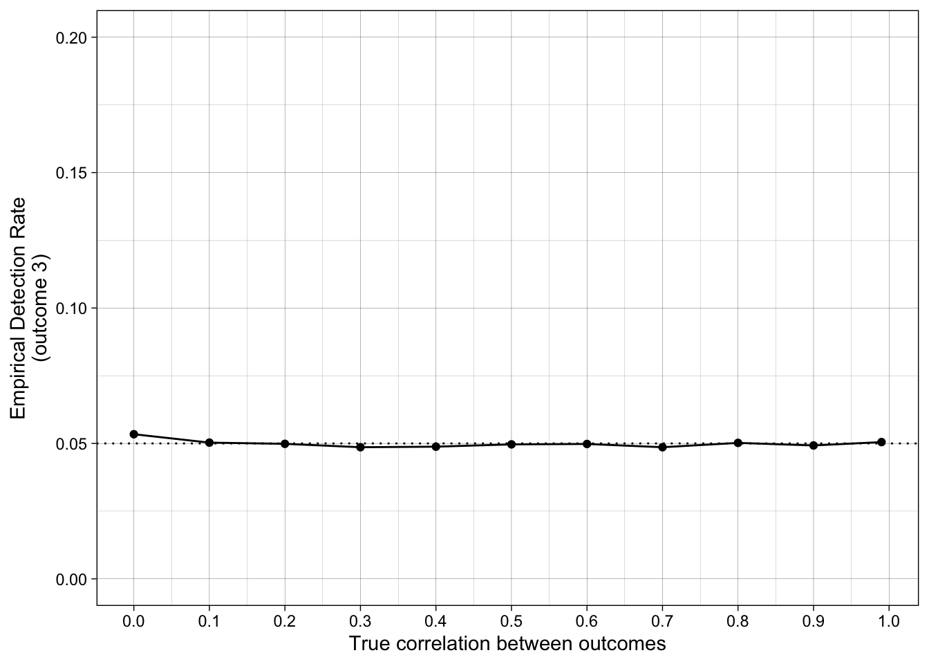
ggplot(simulation_summary, aes(r_between_outcomes, prop_sig_at_least_one)) +
  geom_hline(yintercept = 0.05, linetype = "dotted") +
  geom_point() +
  geom_line() +
  scale_x_continuous(breaks = breaks_pretty(n = 9), name = "True correlation between outcomes") +
  scale_y_continuous(limits = c(0, .2), breaks = breaks_pretty(n = 5), name = "Empirical Detection Rate\n(at least one outcome significant)") +
  theme_linedraw() +
  scale_color_viridis_d(begin = 0.2, end = 0.8)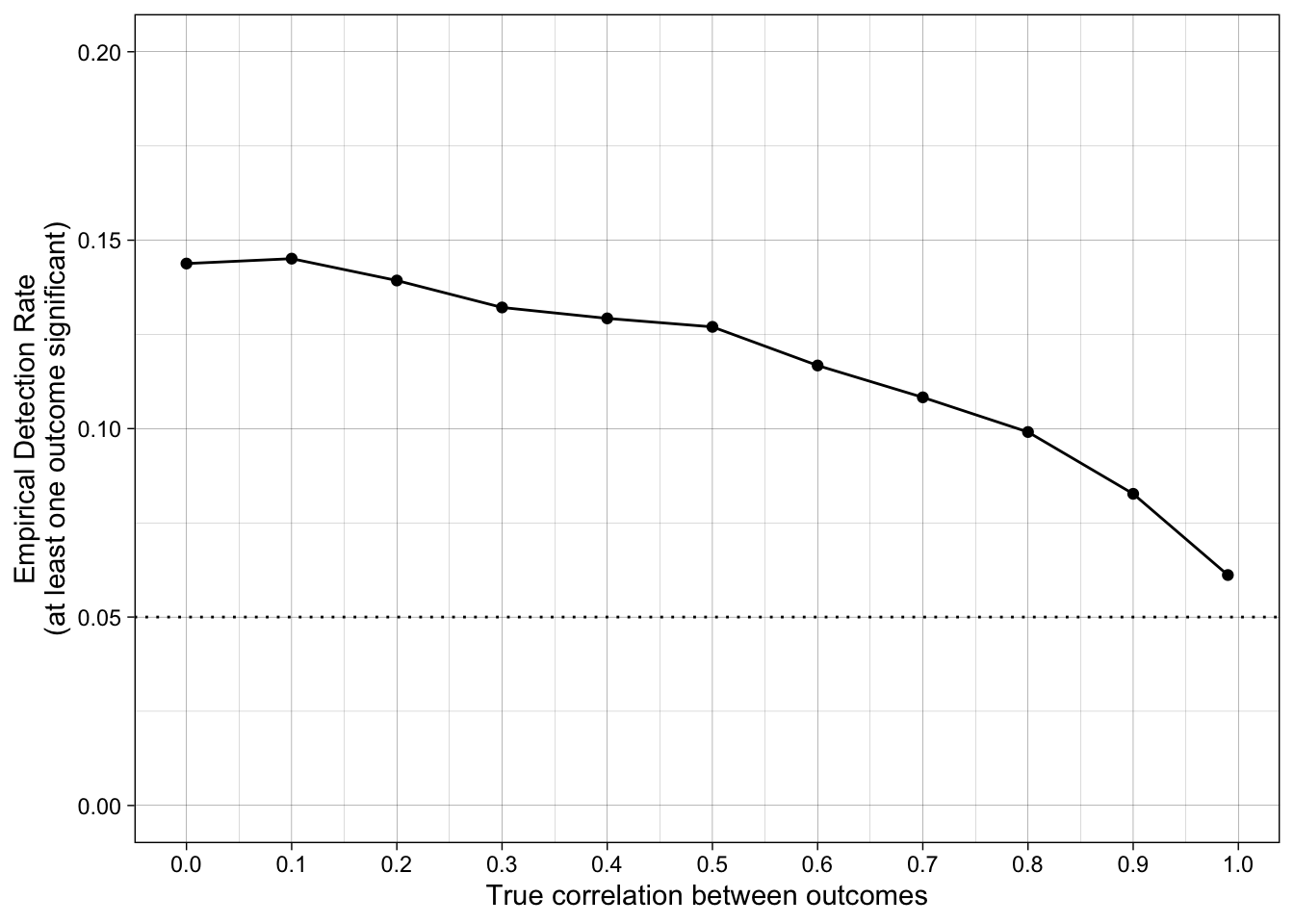
16.4.5 Conclusions
How does the false positive rate change when the outcome measures are correlated?
What perverse incentive does this set up for researchers?
16.5 Check your learning
If authors reported the results of all outcome variables (and not just the ones that ‘worked’):
- Would this problem be improved?
- Would this problem be completely solved?
See the exercises for this chapter for further practice.
16.6 Readings
- Stefan, A. M. and Schönbrodt F. D. (2023) Big little lies: a compendium and simulation of p-hacking strategies. Royal Society Open Science. 10220346 http://doi.org/10.1098/rsos.220346