28  Exercises for ‘Estimation’ chapter

# dependencies
library(tidyr)
library(dplyr)
library(furrr) 
library(parameters)
library(stringr)
library(forcats)
library(ggplot2)
library(scales)
library(ggstance)
library(patchwork)
library(janitor)
library(effectsize)
library(ggstance)
library(knitr)
library(kableExtra)

# set up parallelization
plan(multisession)

28.1 Basis simulation

Same as in the chapter.

# functions for simulation
generate_data <- function(n_per_condition,
                          mean_control,
                          mean_intervention,
                          sd) {
  
  data_control <- 
    tibble(condition = "control",
           score = rnorm(n = n_per_condition, mean = mean_control, sd = sd))
  
  data_intervention <- 
    tibble(condition = "intervention",
           score = rnorm(n = n_per_condition, mean = mean_intervention, sd = sd))
  
  data_combined <- 
    bind_rows(data_control,
              data_intervention) |>
    mutate(condition = factor(condition, level = c("intervention", "control")))
  
  return(data_combined)
}

analyse <- function(data){
  fit <- t.test(
    formula = score ~ condition,
    var.equal = TRUE, # students t test: assumes equal variances
    data = data
  )
  
  results <- fit %>%
    model_parameters() %>%
    as_tibble() %>% 
    janitor::clean_names() %>% 
    # create estimand
    mutate(confidence_interval_width = ci_high - ci_low) |>
    # select columns of interest
    select(mean_diff = difference, # for parameter recovery
           ci_low, # plotting
           ci_high, # plotting
           confidence_interval_width) # estimand
  
  return(results)
}

# simulation parameters
experiment_parameters <- expand_grid(
  n_per_condition = seq(from = 10, to = 100, by = 10),
  mean_control = 4,
  mean_intervention = 5,
  sd = 1.5,
  iteration = 1:1000
) 

# set seed
set.seed(43)

# run simulation
simulation <- experiment_parameters |>
  mutate(generated_data = future_pmap(.l = list(n_per_condition = n_per_condition, 
                                                mean_control = mean_control,
                                                mean_intervention = mean_intervention,
                                                sd = sd),
                                      .f = generate_data,
                                      .progress = TRUE,
                                      .options = furrr_options(seed = TRUE))) |>
  mutate(results = future_pmap(.l = list(data = generated_data),
                               .f = analyse,
                               .progress = TRUE,
                               .options = furrr_options(seed = TRUE)))

# summarise results
results_summary <- simulation |>
  unnest(results) |>
  group_by(n_per_condition) |>
  summarize(mean_difference_in_means = mean(mean_diff),
            mean_ci_low = mean(ci_low),
            mean_ci_high = mean(ci_high),
            mean_confidence_interval_width = mean(confidence_interval_width))

## table
## remember: only round results as you're about to print a table
results_summary |>
  mutate_if(is.numeric, round, digits = 1)

n_per_condition	mean_difference_in_means	mean_ci_low	mean_ci_high	mean_confidence_interval_width
10	1	-0.4	2.4	2.8
20	1	0.0	1.9	1.9
30	1	0.2	1.8	1.5
40	1	0.3	1.7	1.3
50	1	0.4	1.6	1.2
60	1	0.5	1.5	1.1
70	1	0.5	1.5	1.0
80	1	0.5	1.5	0.9
90	1	0.6	1.4	0.9
100	1	0.6	1.4	0.8

## Difference-in-means
ggplot(results_summary, aes(n_per_condition*2, mean_difference_in_means)) +
  geom_point() +
  geom_linerange(aes(ymin = mean_ci_low, ymax = mean_ci_high)) +
  geom_hline(yintercept = 0, linetype = "dotted") +
  scale_x_continuous(breaks = breaks_pretty(n = 10),
                     name = "Total sample size per study") +
  scale_y_continuous(breaks = breaks_pretty(n = 5),
                     #limits = c(0,1),
                     name = "Mean sample difference-in-means\n(and mean 95% CIs)") +
  theme_linedraw() +
  ggtitle("Population difference-in-means = 1")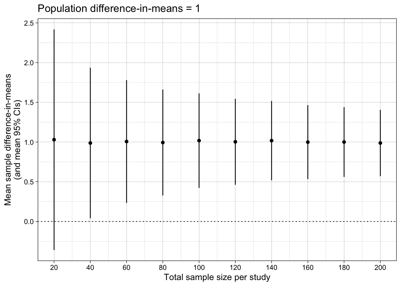

## Difference-in-means' 95% Confidence Interval width
ggplot(results_summary, aes(n_per_condition*2, mean_confidence_interval_width)) +
  geom_hline(yintercept = 0, linetype = "dotted") +
  #geom_linerange(aes(ymin = min_ci_width, ymax = max_ci_width)) +
  geom_point() +
  #scale_y_continuous(name = "95% CI width\n(mean [min, max])", limits = c(0, NA)) +
  scale_y_continuous(name = "Mean sample 95% CI width", 
                     limits = c(0, NA)) +
  scale_x_continuous(breaks = breaks_pretty(n = 9), 
                     name = "Total sample size per study") +
  theme_linedraw() +
  scale_color_viridis_d(begin = 0.3, end = 0.7) +
  ggtitle("Population Mean difference = 1")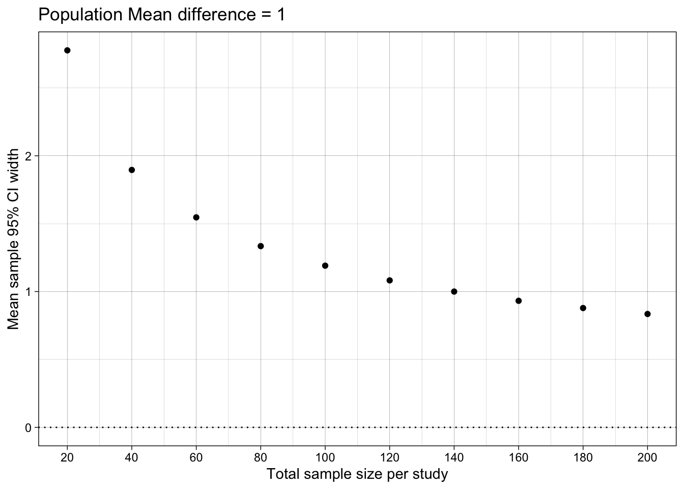

28.2 Exercises

For each of the exercises below, create a copy of the simulation above. Modify it appropriately to answer the exercise.

28.2.1 For each sample size, what proportion of the 95% Confidence Intervals exclude 0?

Use between().

28.2.2 When the population difference in means is 1, what proportion of the p values are statistically significant for each sample size?

Also have the analysis extract a p-value for the difference in means.

Think about it: what statistical property does this represent?

28.2.3 What is the relationship between the confidence interval excluding 0 and the significance of the p value?

For each iteration, calculate if (95% CI!=0) == (p<.05)

28.2.4 When the population difference in means is 0, what proportion of the p values are statistically significant for each sample size?

Change the population effect difference-in-means to zero.

Think about it: what statistical property does this represent?