20  Regression assumes causality ✎ Very rough draft

20.1 Dependencies

library(tidyr)
library(dplyr)
library(purrr) 
library(parameters)
library(lavaan)
library(semPlot)

20.2 Functions

generate_data <- function(n, population_model) {
  
  data <- lavaan::simulateData(model = population_model, sample.nobs = n) 
  
  return(data)
}

analyse <- function(data, model) {
  
  # specify and fit model
  fit <- sem(model = model, data = data)
  #fit <- lm(formula = mode, data = data)
  
  # extract regression beta estimates 
  results <- parameters::model_parameters(fit, standardize = FALSE) |>
    filter(To == "Y" & From == "X") |>  # this corresponds to the Y ~ X effect
    select(beta = Coefficient,
           ci_lower = CI_low,
           ci_upper = CI_high,
           p) 
  
  return(results)
}

 plots_causal <- function(model){
  generate_data(n = 300, population_model = model) %>%
    sem(model = model, data = .) |>
    semPaths(whatLabels = "diagram", 
             layout = layout_matrix, 
             residuals = FALSE,
             edge.label.cex = 1.2, 
             sizeMan = 10)
}

20.3 Does regression assume causality?

20.3.1 Plots

Simple regression: X causes Y

# simple regression
layout_matrix <- matrix(c( 1,  0,
                           -1,  0), 
                        ncol = 2, 
                        byrow = TRUE)

plots_causal("Y ~ 0.5*X")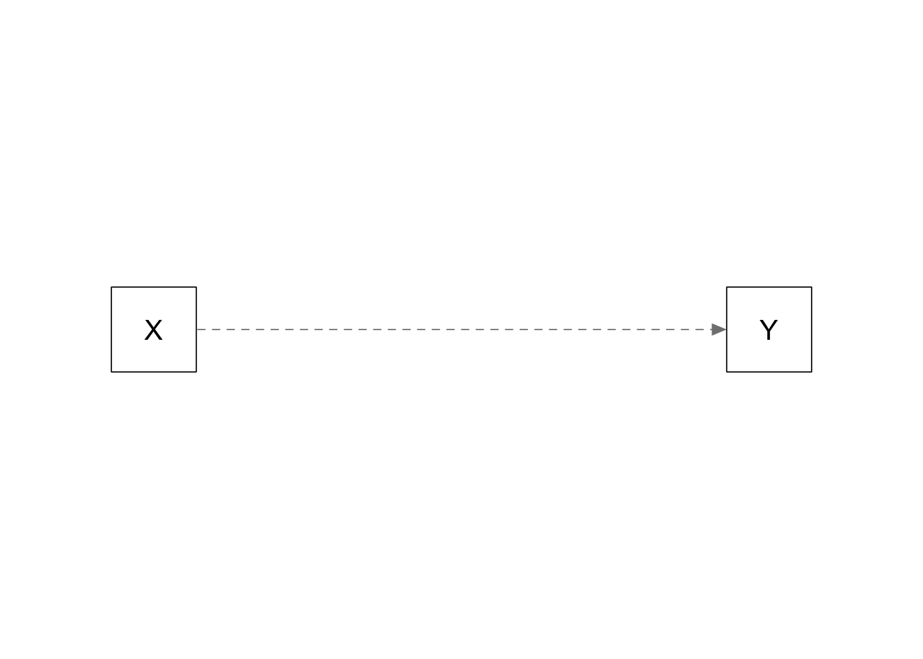

Simple regression: Y causes X

# simple regression
layout_matrix <- matrix(c(-1,  0,
                           1,  0), 
                        ncol = 2, 
                        byrow = TRUE)

plots_causal("X ~ 0.5*Y")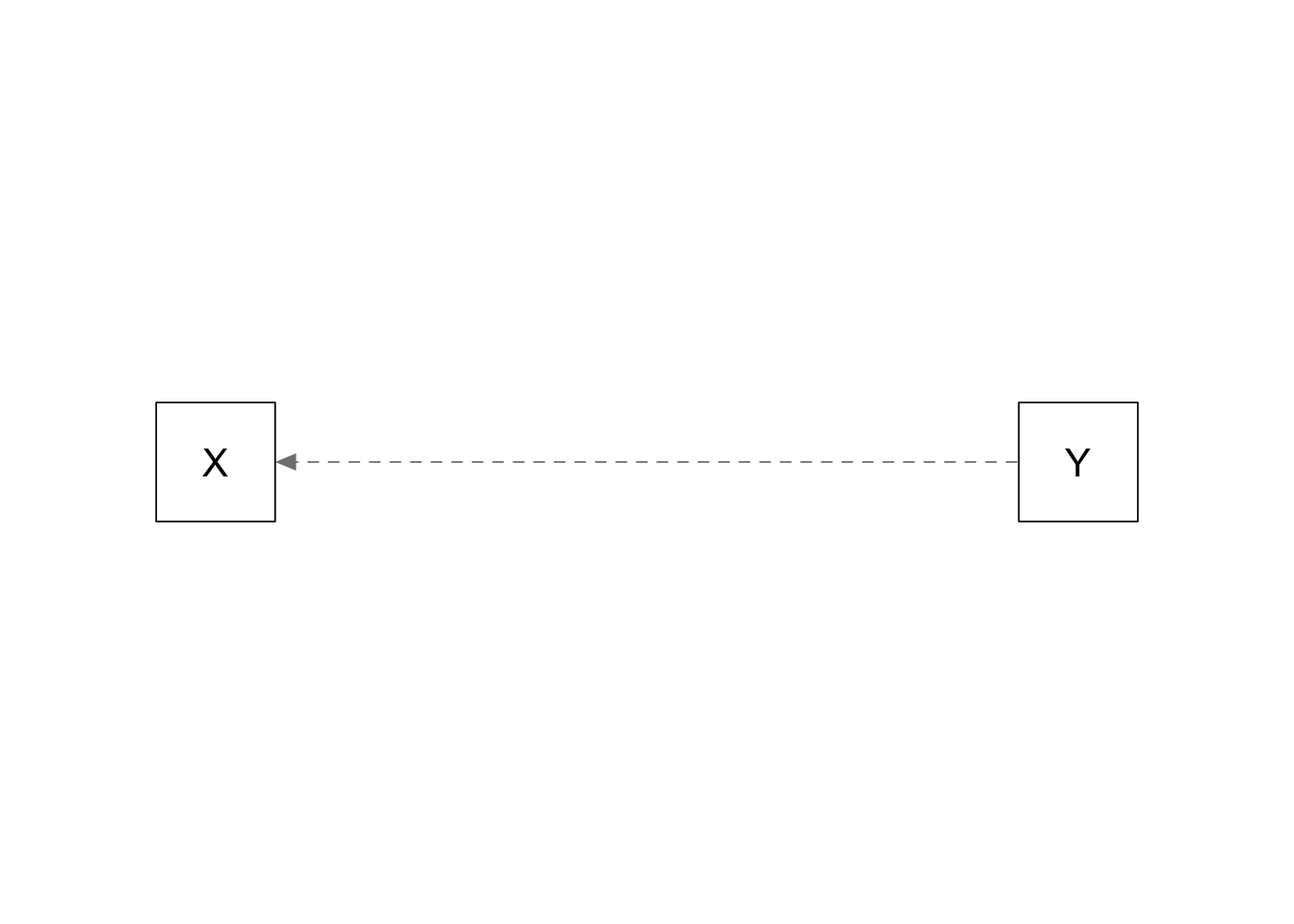

20.3.2 Run simulation

experiment_parameters_grid <- expand_grid(
  n = 200,
  population_model = c("Y ~ 0.5*X",
                       "X ~ 0.5*Y"),
  analyse_model = "Y ~ X",
  iteration = 1:1000
) 

set.seed(42)

simulation <- 
  # using the experiment parameters...
  experiment_parameters_grid |>
  
  # ...generate data... 
  mutate(generated_data = pmap(list(n = n,
                                    population_model = population_model),
                               generate_data)) |>
  # ...analyze data 
  mutate(results = pmap(list(data = generated_data,
                             model = analyse_model),
                        analyse))

20.3.3 Summarize results

simulation_summary <- simulation |>
  unnest(results) |>
  group_by(n,
           population_model,
           analyse_model) |>
  summarize(mean_beta = mean(beta),
            proportion_signficiant = mean(p < .05))

simulation_summary |>
  mutate_if(is.numeric, janitor::round_half_up, digits = 2)

n	population_model	analyse_model	mean_beta	proportion_signficiant
200	X ~ 0.5*Y	Y ~ X	0.4	1
200	Y ~ 0.5*X	Y ~ X	0.5	1

20.4 Collider

20.4.1 Plots

Covariate is a confounder:

layout_matrix <- matrix(c( 1,  0,
                           -1,  0,
                           0,  1), 
                        ncol = 2, 
                        byrow = TRUE)

plots_causal("Y ~ 0.0*X + 0.5*C; X ~ 0.5*C")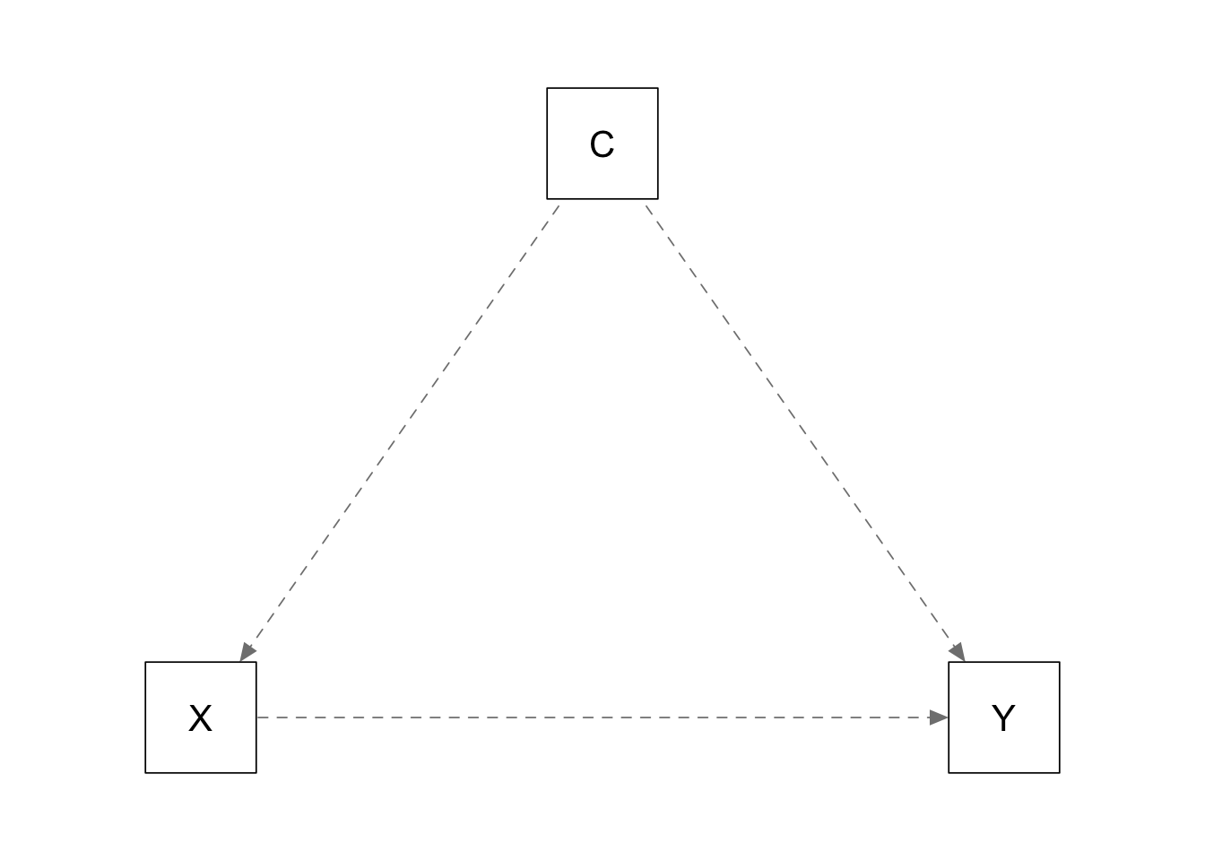

Confounder is a collider:

layout_matrix <- matrix(c( 0,  1,
                           1,  0,
                           -1,  0), 
                        ncol = 2, 
                        byrow = TRUE)

plots_causal("C ~ 0.5*X + 0.5*Y; Y ~ 0.0*X")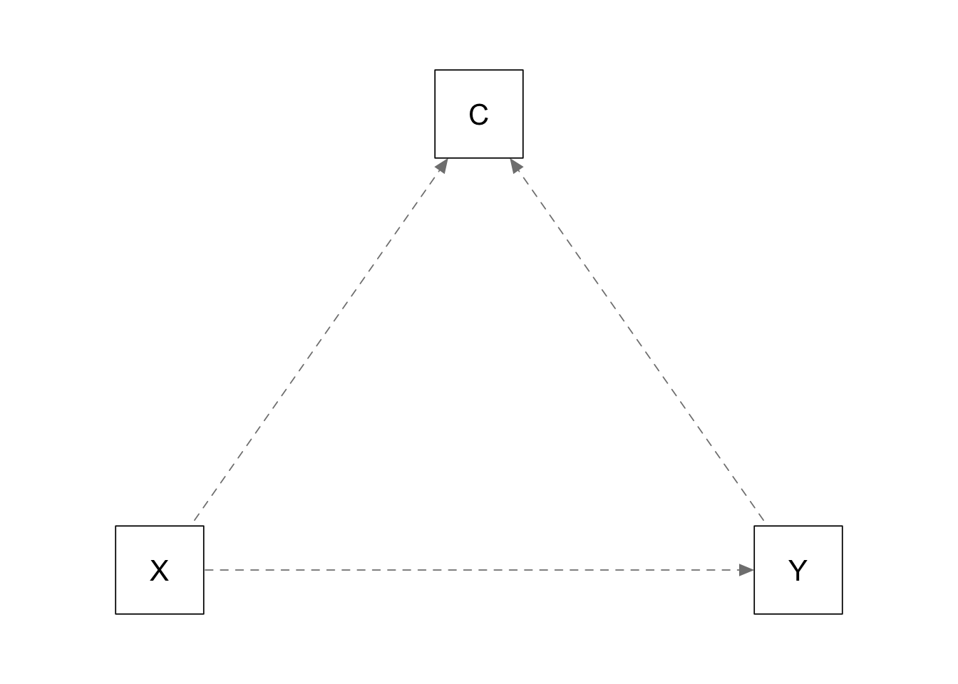

20.4.2 Run simulation

experiment_parameters_grid <- expand_grid(
  n = 200,
  population_model = c("Y ~ 0.5*X + 0.0*C",
                       "C ~ 0.5*X + 0.5*Y; Y ~~ 0.0*X"),
  analyse_model = "Y ~ X + C",
  iteration = 1:1000
)

set.seed(42)

simulation <- 
  # using the experiment parameters...
  experiment_parameters_grid |>
  
  # ...generate data...
  mutate(generated_data = pmap(list(n = n,
                                    population_model = population_model),
                               generate_data)) |>
  # ...analyze data
  mutate(results = pmap(list(data = generated_data,
                             model = analyse_model),
                        analyse))

20.4.3 Summarize results

simulation_summary <- simulation |>
  unnest(results) |>
  group_by(n,
           population_model,
           analyse_model) |>
  summarize(mean_beta = mean(beta),
            proportion_signficiant = mean(p < .05))

simulation_summary |>
  mutate_if(is.numeric, janitor::round_half_up, digits = 2)

n	population_model	analyse_model	mean_beta	proportion_signficiant
200	C ~ 0.5X + 0.5Y; Y ~~ 0.0*X	Y ~ X + C	-0.2	0.82
200	Y ~ 0.5X + 0.0C	Y ~ X + C	0.5	1.00